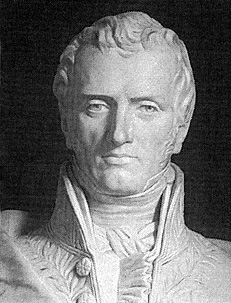
Legendre transformation

Definition in one-dimensional real space

Let ${\displaystyle I\subset \mathbb {R} }$ be an interval, and ${\displaystyle f:I\to \mathbb {R} }$ a convex function; then the Legendre transformof${\displaystyle f}$ is the function ${\displaystyle f^{*}:I^{*}\to \mathbb {R} }$ defined by $${\displaystyle f^{*}(x^{*})=\sup _{x\in I}(x^{*}x-f(x)),\ \ \ \ I^{*}=\left\{x^{*}\in \mathbb {R} :f^{*}(x^{*})<\infty \right\}~}$$ where ${\textstyle \sup }$ denotes the supremum over ${\displaystyle I}$, e.g., ${\textstyle x}$ in ${\textstyle I}$ is chosen such that ${\textstyle x^{*}x-f(x)}$ is maximized at each ${\textstyle x^{*}}$, or ${\textstyle x^{*}}$ is such that ${\displaystyle x^{*}x-f(x)}$ as a bounded value throughout ${\textstyle x}$ exists (e.g., when ${\displaystyle f(x)}$ is a linear function).

The function ${\displaystyle f^{*}}$ is called the convex conjugate function of ${\displaystyle f}$. For historical reasons (rooted in analytic mechanics), the conjugate variable is often denoted ${\displaystyle p}$, instead of ${\displaystyle x^{*}}$. If the convex function ${\displaystyle f}$ is defined on the whole line and is everywhere differentiable, then $${\displaystyle f^{*}(p)=\sup _{x\in I}(px-f(x))=\left(px-f(x)\right)|_{x=(f')^{-1}(p)}}$$ can be interpreted as the negative of the ${\displaystyle y}$-intercept of the tangent line to the graph of ${\displaystyle f}$ that has slope ${\displaystyle p}$.

Definition in n-dimensional real space

The generalization to convex functions ${\displaystyle f:X\to \mathbb {R} }$ on a convex set ${\displaystyle X\subset \mathbb {R} ^{n}}$ is straightforward: ${\displaystyle f^{*}:X^{*}\to \mathbb {R} }$ has domain $${\displaystyle X^{*}=\left\{x^{*}\in \mathbb {R} ^{n}:\sup _{x\in X}(\langle x^{*},x\rangle -f(x))<\infty \right\}}$$ and is defined by $${\displaystyle f^{*}(x^{*})=\sup _{x\in X}(\langle x^{*},x\rangle -f(x)),\quad x^{*}\in X^{*}~,}$$ where ${\displaystyle \langle x^{*},x\rangle }$ denotes the dot product of ${\displaystyle x^{*}}$ and ${\displaystyle x}$.

The Legendre transformation is an application of the duality relationship between points and lines. The functional relationship specified by ${\displaystyle f}$ can be represented equally well as a set of ${\displaystyle (x,y)}$ points, or as a set of tangent lines specified by their slope and intercept values.

Understanding the Legendre transform in terms of derivatives

For a differentiable convex function ${\displaystyle f}$ on the real line with the first derivative ${\displaystyle f'}$ and its inverse ${\displaystyle (f')^{-1}}$, the Legendre transform of ${\displaystyle f}$, ${\displaystyle f^{*}}$, can be specified, up to an additive constant, by the condition that the functions' first derivatives are inverse functions of each other, i.e., ${\displaystyle f'=((f^{*})')^{-1}}$ and ${\displaystyle (f^{*})'=(f')^{-1}}$.

To see this, first note that if ${\displaystyle f}$ as a convex function on the real line is differentiable and ${\displaystyle {\overline {x}}}$ is a critical point of the function of ${\displaystyle x\mapsto p\cdot x-f(x)}$, then the supremum is achieved at ${\textstyle {\overline {x}}}$ (by convexity, see the first figure in this Wikipedia page). Therefore, the Legendre transform of ${\displaystyle f}$ is ${\displaystyle f^{*}(p)=p\cdot {\overline {x}}-f({\overline {x}})}$.

Then, suppose that the first derivative ${\displaystyle f'}$ is invertible and let the inverse be ${\displaystyle g=(f')^{-1}}$. Then for each ${\textstyle p}$, the point ${\displaystyle g(p)}$ is the unique critical point ${\textstyle {\overline {x}}}$ of the function ${\displaystyle x\mapsto px-f(x)}$ (i.e., ${\displaystyle {\overline {x}}=g(p)}$) because ${\displaystyle f'(g(p))=p}$ and the function's first derivative with respect to ${\displaystyle x}$ at ${\displaystyle g(p)}$ is ${\displaystyle p-f'(g(p))=0}$. Hence we have ${\displaystyle f^{*}(p)=p\cdot g(p)-f(g(p))}$ for each ${\textstyle p}$. By differentiating with respect to ${\textstyle p}$, we find $${\displaystyle (f^{*})'(p)=g(p)+p\cdot g'(p)-f'(g(p))\cdot g'(p).}$$ Since ${\displaystyle f'(g(p))=p}$ this simplifies to ${\displaystyle (f^{*})'(p)=g(p)=(f')^{-1}(p)}$. In other words, ${\displaystyle (f^{*})'}$ and ${\displaystyle f'}$ are inverses to each other.

In general, if ${\displaystyle h'=(f')^{-1}}$ as the inverse of ${\displaystyle f',}$ then ${\displaystyle h'=(f^{*})'}$ so integration gives ${\displaystyle f^{*}=h+c.}$ with a constant ${\displaystyle c.}$

In practical terms, given ${\displaystyle f(x),}$ the parametric plot of ${\displaystyle xf'(x)-f(x)}$ versus ${\displaystyle f'(x)}$ amounts to the graph of ${\displaystyle f^{*}(p)}$ versus ${\displaystyle p.}$

In some cases (e.g. thermodynamic potentials, below), a non-standard requirement is used, amounting to an alternative definition of f * with a minus sign, $${\displaystyle f(x)-f^{*}(p)=xp.}$$

Formal definition in physics context

In analytical mechanics and thermodynamics, Legendre transformation is usually defined as follows: suppose ${\displaystyle f}$ is a function of ${\displaystyle x,}$ then we have

${\displaystyle \mathrm {d} f={\frac {\mathrm {d} f}{\mathrm {d} x}}\mathrm {d} x.}$

performing Legendre transformation on this function means that we take ${\displaystyle p={\frac {\mathrm {d} f}{\mathrm {d} x}}}$ as the independent variable, so that the above expression can be written as

${\displaystyle \mathrm {d} f=p\mathrm {d} x,}$

and according to Leibniz's rule ${\displaystyle \mathrm {d} (uv)=u\mathrm {d} v+v\mathrm {d} u,}$ then we have

${\displaystyle \mathrm {d} \left(xp-f\right)=x\mathrm {d} p,}$

and taking ${\displaystyle f^{*}=xp-f,}$ we have ${\displaystyle \mathrm {d} f^{*}=x\mathrm {d} p,}$ which means

${\displaystyle {\frac {\mathrm {d} f^{*}}{\mathrm {d} p}}=x.}$

When ${\displaystyle f}$ is a function of ${\displaystyle n}$ variables ${\displaystyle x_{1},x_{2},\cdots ,x_{n}}$, then we can perform the Legendre transformation on each one or several variables: we have

${\displaystyle \mathrm {d} f=p_{1}\mathrm {d} x_{1}+p_{2}\mathrm {d} x_{2}+\cdots +p_{n}\mathrm {d} x_{n}}$

where ${\displaystyle p_{i}={\frac {\partial f}{\partial x_{i}}}.}$ Then if we want to perform Legendre transformation on, e.g. ${\displaystyle x_{1}}$ then we take ${\displaystyle p_{1}}$ together with ${\displaystyle x_{2},\cdots ,x_{n}}$ as independent variables, and with Leibniz's rule we have

${\displaystyle \mathrm {d} (f-x_{1}p_{1})=-x_{1}\mathrm {d} p_{1}+p_{2}\mathrm {d} x_{2}+\cdots +p_{n}\mathrm {d} x_{n}.}$

so for function ${\displaystyle \varphi (p_{1},x_{2},\cdots ,x_{n})=f(x_{1},x_{2},\cdots ,x_{n})-x_{1}p_{1},}$ we have

${\displaystyle {\frac {\partial \varphi }{\partial p_{1}}}=-x_{1},\quad {\frac {\partial \varphi }{\partial x_{2}}}=p_{2},\quad \cdots ,\quad {\frac {\partial \varphi }{\partial x_{n}}}=p_{n}.}$

We can also do this transformation for variables ${\displaystyle x_{2},\cdots ,x_{n}}$. If we do it to all the variables, then we have

${\displaystyle \mathrm {d} \varphi =-x_{1}\mathrm {d} p_{1}-x_{2}\mathrm {d} p_{2}-\cdots -x_{n}\mathrm {d} p_{n}}$ where ${\displaystyle \varphi =f-x_{1}p_{1}-x_{2}p_{2}-\cdots -x_{n}p_{n}.}$

In analytical mechanics, people perform this transformation on variables ${\displaystyle {\dot {q}}_{1},{\dot {q}}_{2},\cdots ,{\dot {q}}_{n}}$ of the Lagrangian ${\displaystyle L(q_{1},\cdots ,q_{n},{\dot {q}}_{1},\cdots ,{\dot {q}}_{n})}$ to get the Hamiltonian:

${\displaystyle H(q_{1},\cdots ,q_{n},p_{1},\cdots ,p_{n})=\sum _{i=1}^{n}p_{i}{\dot {q}}_{i}-L(q_{1},\cdots ,q_{n},{\dot {q}}_{1}\cdots ,{\dot {q}}_{n})}$

and in thermodynamics, people perform this transformation on variables according to the type of thermodynamic system they want. E.g. starting from the cardinal function of state, the internal energy ${\displaystyle U(S,V)}$, we have

${\displaystyle \mathrm {d} U=T\mathrm {d} S-p\mathrm {d} V,}$

we can perform Legendre transformation on either or both of ${\displaystyle S,V}$ yielding

${\displaystyle \mathrm {d} H=\mathrm {d} (U+pV)\ \ \ \ \ \ \ \ \ \ =\ \ \ \ T\mathrm {d} S+V\mathrm {d} p}$

${\displaystyle \mathrm {d} F=\mathrm {d} (U-TS)\ \ \ \ \ \ \ \ \ \ =-S\mathrm {d} T-p\mathrm {d} V}$

${\displaystyle \mathrm {d} G=\mathrm {d} (U-TS+pV)=-S\mathrm {d} T+V\mathrm {d} p}$

and each of these three expressions has a physical meaning.

This definition of Legendre transformation is the one originally introduced by Legendre in his work in 1787, ^[1] and still applied by physicists nowadays. Indeed, this definition can be mathematically rigorous if we treat all the variables and functions defined above, e.g. ${\displaystyle f,x_{1},\cdots ,x_{n},p_{1},\cdots ,p_{n},}$ as differentiable functions defined on an open set of ${\displaystyle \mathbb {R} ^{n}}$ or on a differentiable manifold, and ${\displaystyle \mathrm {d} f,\mathrm {d} x_{i},\mathrm {d} p_{i}}$ their differentials (which are treated as cotangent vector field in the context of differentiable manifold). And this definition is equivalent to the modern mathematicians' definition as long as ${\displaystyle f}$ is differentiable and convex for the variables ${\displaystyle x_{1},x_{2},\cdots ,x_{n}.}$

Example 1

Consider the exponential function ${\displaystyle f(x)=e^{x},}$ which has the domain ${\displaystyle I=\mathbb {R} }$. From the definition, the Legendre transform is $${\displaystyle f^{*}(x^{*})=\sup _{x\in \mathbb {R} }(x^{*}x-e^{x}),\quad x^{*}\in I^{*}}$$ where ${\displaystyle I^{*}}$ remains to be determined. To evaluate the supremum, compute the derivative of ${\displaystyle x^{*}x-e^{x}}$ with respect to ${\displaystyle x}$ and set equal to zero: $${\displaystyle {\frac {d}{dx}}(x^{*}x-e^{x})=x^{*}-e^{x}=0.}$$ The second derivative ${\displaystyle -e^{x}}$ is negative everywhere, so the maximal value is achieved at ${\displaystyle x=\ln(x^{*})}$. Thus, the Legendre transform is $${\displaystyle f^{*}(x^{*})=x^{*}\ln(x^{*})-e^{\ln(x^{*})}=x^{*}(\ln(x^{*})-1)}$$ and has domain ${\displaystyle I^{*}=(0,\infty ).}$ This illustrates that the domains of a function and its Legendre transform can be different.

To find the Legendre transformation of the Legendre transformation of ${\displaystyle f}$, $${\displaystyle f^{**}(x)=\sup _{x^{*}\in \mathbb {R} }(xx^{*}-x^{*}(\ln(x^{*})-1)),\quad x\in I,}$$ where a variable ${\displaystyle x}$ is intentionally used as the argument of the function ${\displaystyle f^{**}}$ to show the involution property of the Legendre transform as ${\displaystyle f^{**}=f}$. we compute $${\displaystyle {\begin{aligned}0&={\frac {d}{dx^{*}}}{\big (}xx^{*}-x^{*}(\ln(x^{*})-1){\big )}=x-\ln(x^{*})\end{aligned}}}$$ thus the maximum occurs at ${\displaystyle x^{*}=e^{x}}$ because the second derivative ${\displaystyle {\frac {d^{2}}{{dx^{*}}^{2}}}f^{**}(x)=-{\frac {1}{x^{*}}}<0}$ over the domain of ${\displaystyle f^{**}}$ as ${\displaystyle I^{*}=(0,\infty ).}$ As a result, ${\displaystyle f^{**}}$ is found as $${\displaystyle {\begin{aligned}f^{**}(x)&=xe^{x}-e^{x}(\ln(e^{x})-1)=e^{x},\end{aligned}}}$$ thereby confirming that ${\displaystyle f=f^{**},}$ as expected.

Example 2

Let f(x) = cx² defined on R, where c > 0 is a fixed constant.

For x* fixed, the function of x, x*x − f(x) = x*x − cx² has the first derivative x* − 2cx and second derivative −2c; there is one stationary point at x = x*/2c, which is always a maximum.

Thus, I* = R and $${\displaystyle f^{*}(x^{*})={\frac {{x^{*}}^{2}}{4c}}~.}$$

The first derivatives of f, 2cx, and of f *, x*/(2c), are inverse functions to each other. Clearly, furthermore, $${\displaystyle f^{**}(x)={\frac {1}{4(1/4c)}}x^{2}=cx^{2}~,}$$ namely f ** = f.

Example 3

Let f(x) = x² for x ∈ (I = [2, 3]).

For x* fixed, x*x − f(x) is continuous on I compact, hence it always takes a finite maximum on it; it follows that the domain of the Legendre transform of ${\displaystyle f}$ is I* = R.

The stationary point at x = x*/2 (found by setting that the first derivative of x*x − f(x) with respect to ${\displaystyle x}$ equal to zero) is in the domain [2, 3] if and only if 4 ≤ x* ≤ 6. Otherwise the maximum is taken either at x = 2 or x = 3 because the second derivative of x*x − f(x) with respect to ${\displaystyle x}$ is negative as ${\displaystyle -2}$; for a part of the domain ${\displaystyle x^{*}<4}$ the maximum that x*x − f(x) can take with respect to ${\displaystyle x\in [2,3]}$ is obtained at ${\displaystyle x=2}$ while for ${\displaystyle x^{*}>6}$ it becomes the maximum at ${\displaystyle x=3}$. Thus, it follows that $${\displaystyle f^{*}(x^{*})={\begin{cases}2x^{*}-4,&x^{*}<4\\{\frac {{x^{*}}^{2}}{4}},&4\leq x^{*}\leq 6,\\3x^{*}-9,&x^{*}>6.\end{cases}}}$$

Example 4

The function f(x) = cx is convex, for every x (strict convexity is not required for the Legendre transformation to be well defined). Clearly x*x − f(x) = (x* − c)x is never bounded from above as a function of x, unless x* − c = 0. Hence f* is defined on I* = {c} and f*(c) = 0. (The definition of the Legendre transform requires the existence of the supremum, that requires upper bounds.)

One may check involutivity: of course, x*x − f*(x*) is always bounded as a function of x*∈{c}, hence I** = R. Then, for all x one has $${\displaystyle \sup _{x^{*}\in \{c\}}(xx^{*}-f^{*}(x^{*}))=xc,}$$ and hence f **(x) = cx = f(x).

Example 5

As an example of a convex continuous function that is not everywhere differentiable, consider ${\displaystyle f(x)=|x|}$. This gives$${\displaystyle f^{*}(x^{*})=\sup _{x}(xx^{*}-|x|)=\max \left(\sup _{x\geq 0}x(x^{*}-1),\,\sup _{x\leq 0}x(x^{*}+1)\right),}$$and thus ${\displaystyle f^{*}(x^{*})=0}$ on its domain ${\displaystyle I^{*}=[-1,1]}$.

Example 6: several variables

Let $${\displaystyle f(x)=\langle x,Ax\rangle +c}$$ be defined on X = Rⁿ, where A is a real, positive definite matrix.

Then f is convex, and $${\displaystyle \langle p,x\rangle -f(x)=\langle p,x\rangle -\langle x,Ax\rangle -c,}$$ has gradient p − 2Ax and Hessian −2A, which is negative; hence the stationary point x = A⁻¹p/2 is a maximum.

We have X* = Rⁿ, and $${\displaystyle f^{*}(p)={\frac {1}{4}}\langle p,A^{-1}p\rangle -c.}$$

Analytical mechanics

A Legendre transform is used in classical mechanics to derive the Hamiltonian formulation from the Lagrangian formulation, and conversely. A typical Lagrangian has the form

$${\displaystyle L(v,q)={\tfrac {1}{2}}\langle v,Mv\rangle -V(q),}$$ where ${\displaystyle (v,q)}$ are coordinates on Rⁿ × Rⁿ, M is a positive definite real matrix, and $${\displaystyle \langle x,y\rangle =\sum _{j}x_{j}y_{j}.}$$

For every q fixed, ${\displaystyle L(v,q)}$ is a convex function of ${\displaystyle v}$, while ${\displaystyle V(q)}$ plays the role of a constant.

Hence the Legendre transform of ${\displaystyle L(v,q)}$ as a function of ${\displaystyle v}$ is the Hamiltonian function, $${\displaystyle H(p,q)={\tfrac {1}{2}}\langle p,M^{-1}p\rangle +V(q).}$$

In a more general setting, ${\displaystyle (v,q)}$ are local coordinates on the tangent bundle ${\displaystyle T{\mathcal {M}}}$ of a manifold ${\displaystyle {\mathcal {M}}}$. For each q, ${\displaystyle L(v,q)}$ is a convex function of the tangent space V_q. The Legendre transform gives the Hamiltonian ${\displaystyle H(p,q)}$ as a function of the coordinates (p, q) of the cotangent bundle ${\displaystyle T^{*}{\mathcal {M}}}$; the inner product used to define the Legendre transform is inherited from the pertinent canonical symplectic structure. In this abstract setting, the Legendre transformation corresponds to the tautological one-form.^{[ further explanation needed ]}

Thermodynamics

The strategy behind the use of Legendre transforms in thermodynamics is to shift from a function that depends on a variable to a new (conjugate) function that depends on a new variable, the conjugate of the original one. The new variable is the partial derivative of the original function with respect to the original variable. The new function is the difference between the original function and the product of the old and new variables. Typically, this transformation is useful because it shifts the dependence of, e.g., the energy from an extensive variable to its conjugate intensive variable, which can often be controlled more easily in a physical experiment.

For example, the internal energy U is an explicit function of the extensive variables entropy S, volume V, and chemical composition N_i (e.g., ${\displaystyle i=1,2,3,\ldots }$) $${\displaystyle U=U\left(S,V,\{N_{i}\}\right),}$$ which has a total differential $${\displaystyle dU=T\,dS-P\,dV+\sum \mu _{i}\,dN_{i}}$$

where ${\displaystyle T=\left.{\frac {\partial U}{\partial S}}\right\vert _{V,N_{i\ for\ all\ i\ values}},P=\left.-{\frac {\partial U}{\partial V}}\right\vert _{S,N_{i\ for\ all\ i\ values}},\mu _{i}=\left.{\frac {\partial U}{\partial N_{i}}}\right\vert _{S,V,N_{j\ for\ all\ j\neq i}}}$.

(Subscripts are not necessary by the definition of partial derivatives but left here for clarifying variables.) Stipulating some common reference state, by using the (non-standard) Legendre transform of the internal energy U with respect to volume V, the enthalpy H may be obtained as the following.

To get the (standard) Legendre transform ${\textstyle U^{*}}$ of the internal energy U with respect to volume V, the function ${\textstyle u\left(p,S,V,\{{{N}_{i}}\}\right)=pV-U}$ is defined first, then it shall be maximized or bounded by V. To do this, the condition ${\textstyle {\frac {\partial u}{\partial V}}=p-{\frac {\partial U}{\partial V}}=0\to p={\frac {\partial U}{\partial V}}}$ needs to be satisfied, so ${\textstyle U^{*}={\frac {\partial U}{\partial V}}V-U}$ is obtained. This approach is justified because U is a linear function with respect to V (so a convex function on V) by the definition of extensive variables. The non-standard Legendre transform here is obtained by negating the standard version, so ${\textstyle -U^{*}=H=U-{\frac {\partial U}{\partial V}}V=U+PV}$.

H is definitely a state function as it is obtained by adding PV (P and V as state variables) to a state function ${\textstyle U=U\left(S,V,\{N_{i}\}\right)}$, so its differential is an exact differential. Because of ${\textstyle dH=T\,dS+V\,dP+\sum \mu _{i}\,dN_{i}}$ and the fact that it must be an exact differential, ${\displaystyle H=H(S,P,\{N_{i}\})}$.

The enthalpy is suitable for description of processes in which the pressure is controlled from the surroundings.

It is likewise possible to shift the dependence of the energy from the extensive variable of entropy, S, to the (often more convenient) intensive variable T, resulting in the Helmholtz and Gibbs free energies. The Helmholtz free energy A, and Gibbs energy G, are obtained by performing Legendre transforms of the internal energy and enthalpy, respectively, $${\displaystyle A=U-TS~,}$$$${\displaystyle G=H-TS=U+PV-TS~.}$$

The Helmholtz free energy is often the most useful thermodynamic potential when temperature and volume are controlled from the surroundings, while the Gibbs energy is often the most useful when temperature and pressure are controlled from the surroundings.

Variable capacitor

As another example from physics, consider a parallel conductive plate capacitor, in which the plates can move relative to one another. Such a capacitor would allow transfer of the electric energy which is stored in the capacitor into external mechanical work, done by the force acting on the plates. One may think of the electric charge as analogous to the "charge" of a gas in a cylinder, with the resulting mechanical force exerted on a piston.

Compute the force on the plates as a function of x, the distance which separates them. To find the force, compute the potential energy, and then apply the definition of force as the gradient of the potential energy function.

The electrostatic potential energy stored in a capacitor of the capacitance C(x) and a positive electric charge +Q or negative charge -Q on each conductive plate is (with using the definition of the capacitance as ${\textstyle C={\frac {Q}{V}}}$),

$${\displaystyle U(Q,\mathbf {x} )={\frac {1}{2}}QV(Q,\mathbf {x} )={\frac {1}{2}}{\frac {Q^{2}}{C(\mathbf {x} )}},~}$$

where the dependence on the area of the plates, the dielectric constant of the insulation material between the plates, and the separation x are abstracted away as the capacitance C(x). (For a parallel plate capacitor, this is proportional to the area of the plates and inversely proportional to the separation.)

The force F between the plates due to the electric field created by the charge separation is then $${\displaystyle \mathbf {F} (\mathbf {x} )=-{\frac {dU}{d\mathbf {x} }}~.}$$

If the capacitor is not connected to any electric circuit, then the electric charges on the plates remain constant and the voltage varies when the plates move with respect to each other, and the force is the negative gradient of the electrostatic potential energy as $${\displaystyle \mathbf {F} (\mathbf {x} )={\frac {1}{2}}{\frac {dC(\mathbf {x} )}{d\mathbf {x} }}{\frac {Q^{2}}{{C(\mathbf {x} )}^{2}}}={\frac {1}{2}}{\frac {dC(\mathbf {x} )}{d\mathbf {x} }}V(\mathbf {x} )^{2}}$$

where ${\textstyle V(Q,\mathbf {x} )=V(\mathbf {x} )}$ as the charge is fixed in this configuration.

However, instead, suppose that the voltage between the plates V is maintained constant as the plate moves by connection to a battery, which is a reservoir for electric charges at a constant potential difference. Then the amount of charges${\textstyle Q}$is a variable instead of the voltage; ${\textstyle Q}$ and ${\textstyle V}$ are the Legendre conjugate to each other. To find the force, first compute the non-standard Legendre transform ${\textstyle U^{*}}$ with respect to ${\textstyle Q}$ (also with using ${\textstyle C={\frac {Q}{V}}}$),

$${\displaystyle U^{*}=U-\left.{\frac {\partial U}{\partial Q}}\right|_{\mathbf {x} }\cdot Q=U-{\frac {1}{2C(\mathbf {x} )}}\left.{\frac {\partial Q^{2}}{\partial Q}}\right|_{\mathbf {x} }\cdot Q=U-QV={\frac {1}{2}}QV-QV=-{\frac {1}{2}}QV=-{\frac {1}{2}}V^{2}C(\mathbf {x} ).}$$

This transformation is possible because ${\textstyle U}$ is now a linear function of ${\textstyle Q}$ so is convex on it. The force now becomes the negative gradient of this Legendre transform, resulting in the same force obtained from the original function ${\textstyle U}$, $${\displaystyle \mathbf {F} (\mathbf {x} )=-{\frac {dU^{*}}{d\mathbf {x} }}={\frac {1}{2}}{\frac {dC(\mathbf {x} )}{d\mathbf {x} }}V^{2}.}$$

The two conjugate energies ${\textstyle U}$ and ${\textstyle U^{*}}$ happen to stand opposite to each other (their signs are opposite), only because of the linearity of the capacitance—except now Q is no longer a constant. They reflect the two different pathways of storing energy into the capacitor, resulting in, for instance, the same "pull" between a capacitor's plates.

Probability theory

In large deviations theory, the rate function is defined as the Legendre transformation of the logarithm of the moment generating function of a random variable. An important application of the rate function is in the calculation of tail probabilities of sums of i.i.d. random variables, in particular in Cramér's theorem.

If ${\displaystyle X_{n}}$ are i.i.d. random variables, let ${\displaystyle S_{n}=X_{1}+\cdots +X_{n}}$ be the associated random walk and ${\displaystyle M(\xi )}$ the moment generating function of ${\displaystyle X_{1}}$. For ${\displaystyle \xi \in \mathbb {R} }$, ${\displaystyle E[e^{\xi S_{n}}]=M(\xi )^{n}}$. Hence, by Markov's inequality, one has for ${\displaystyle \xi \geq 0}$ and ${\displaystyle a\in \mathbb {R} }$$${\displaystyle P(S_{n}/n>a)\leq e^{-n\xi a}M(\xi )^{n}=\exp[-n(\xi a-\Lambda (\xi ))]}$$ where ${\displaystyle \Lambda (\xi )=\log M(\xi )}$. Since the left-hand side is independent of ${\displaystyle \xi }$, we may take the infimum of the right-hand side, which leads one to consider the supremum of ${\displaystyle \xi a-\Lambda (\xi )}$, i.e., the Legendre transform of ${\displaystyle \Lambda }$, evaluated at ${\displaystyle x=a}$.

Microeconomics

Legendre transformation arises naturally in microeconomics in the process of finding the supply S(P) of some product given a fixed price P on the market knowing the cost function C(Q), i.e. the cost for the producer to make/mine/etc. Q units of the given product.

A simple theory explains the shape of the supply curve based solely on the cost function. Let us suppose the market price for a one unit of our product is P. For a company selling this good, the best strategy is to adjust the production Q so that its profit is maximized. We can maximize the profit $${\displaystyle {\text{profit}}={\text{revenue}}-{\text{costs}}=PQ-C(Q)}$$ by differentiating with respect to Q and solving $${\displaystyle P-C'(Q_{\text{opt}})=0.}$$

Q_opt represents the optimal quantity Q of goods that the producer is willing to supply, which is indeed the supply itself: $${\displaystyle S(P)=Q_{\text{opt}}(P)=(C')^{-1}(P).}$$

If we consider the maximal profit as a function of price, ${\displaystyle {\text{profit}}_{\text{max}}(P)}$, we see that it is the Legendre transform of the cost function ${\displaystyle C(Q)}$.

References

1. 1 2 Legendre, Adrien-Marie (1789). Mémoire sur l'intégration de quelques équations aux différences partielles. In Histoire de l'Académie royale des sciences, avec les mémoires de mathématique et de physique (in French). Vol. 1787. Paris: Imprimerie royale. pp. 309–351.
2. "Legendre Transform | Nick Alger // Maps, art, etc". Archived from the original on 2015-03-12. Retrieved 2011-01-26.
3. 1 2 Ana Cannas da Silva. Lectures on Symplectic Geometry, Corrected 2nd printing. Springer-Verlag, 2008. pp. 147-148. ISBN   978-3-540-42195-5.
Further reading