In statistics, the logistic model is a statistical model that models the log-odds of an event as a linear combination of one or more independent variables. In regression analysis, logistic regression is estimating the parameters of a logistic model. In binary logistic regression there is a single binary dependent variable, coded by an indicator variable, where the two values are labeled "0" and "1", while the independent variables can each be a binary variable or a continuous variable. The corresponding probability of the value labeled "1" can vary between 0 and 1, hence the labeling; the function that converts log-odds to probability is the logistic function, hence the name. The unit of measurement for the log-odds scale is called a logit, from logistic unit, hence the alternative names. See § Background and § Definition for formal mathematics, and § Example for a worked example.

In statistics, an interaction may arise when considering the relationship among three or more variables, and describes a situation in which the effect of one causal variable on an outcome depends on the state of a second causal variable. Although commonly thought of in terms of causal relationships, the concept of an interaction can also describe non-causal associations. Interactions are often considered in the context of regression analyses or factorial experiments.
In statistics, a categorical variable is a variable that can take on one of a limited, and usually fixed, number of possible values, assigning each individual or other unit of observation to a particular group or nominal category on the basis of some qualitative property. In computer science and some branches of mathematics, categorical variables are referred to as enumerations or enumerated types. Commonly, each of the possible values of a categorical variable is referred to as a level. The probability distribution associated with a random categorical variable is called a categorical distribution.
In statistics, multicollinearity or collinearity is a situation where the predictors in a regression model are linearly dependent.

In statistics, the coefficient of determination, denoted R2 or r2 and pronounced "R squared", is the proportion of the variation in the dependent variable that is predictable from the independent variable(s).
In statistics, omitted-variable bias (OVB) occurs when a statistical model leaves out one or more relevant variables. The bias results in the model attributing the effect of the missing variables to those that were included.
In statistics, a linear probability model (LPM) is a special case of a binary regression model. Here the dependent variable for each observation takes values which are either 0 or 1. The probability of observing a 0 or 1 in any one case is treated as depending on one or more explanatory variables. For the "linear probability model", this relationship is a particularly simple one, and allows the model to be fitted by linear regression.

In statistics, ordinary least squares (OLS) is a type of linear least squares method for choosing the unknown parameters in a linear regression model by the principle of least squares: minimizing the sum of the squares of the differences between the observed dependent variable in the input dataset and the output of the (linear) function of the independent variable. Some sources consider OLS to be linear regression.
In digital circuits and machine learning, a one-hot is a group of bits among which the legal combinations of values are only those with a single high (1) bit and all the others low (0). A similar implementation in which all bits are '1' except one '0' is sometimes called one-cold. In statistics, dummy variables represent a similar technique for representing categorical data.
In statistics, Poisson regression is a generalized linear model form of regression analysis used to model count data and contingency tables. Poisson regression assumes the response variable Y has a Poisson distribution, and assumes the logarithm of its expected value can be modeled by a linear combination of unknown parameters. A Poisson regression model is sometimes known as a log-linear model, especially when used to model contingency tables.
The Chow test, proposed by econometrician Gregory Chow in 1960, is a test of whether the true coefficients in two linear regressions on different data sets are equal. In econometrics, it is most commonly used in time series analysis to test for the presence of a structural break at a period which can be assumed to be known a priori. In program evaluation, the Chow test is often used to determine whether the independent variables have different impacts on different subgroups of the population.
In statistics, multinomial logistic regression is a classification method that generalizes logistic regression to multiclass problems, i.e. with more than two possible discrete outcomes. That is, it is a model that is used to predict the probabilities of the different possible outcomes of a categorically distributed dependent variable, given a set of independent variables.
In statistics, binomial regression is a regression analysis technique in which the response has a binomial distribution: it is the number of successes in a series of independent Bernoulli trials, where each trial has probability of success . In binomial regression, the probability of a success is related to explanatory variables: the corresponding concept in ordinary regression is to relate the mean value of the unobserved response to explanatory variables.
In statistics, the variance inflation factor (VIF) is the ratio (quotient) of the variance of a parameter estimate when fitting a full model that includes other parameters to the variance of the parameter estimate if the model is fit with only the parameter on its own. The VIF provides an index that measures how much the variance of an estimated regression coefficient is increased because of collinearity.
In statistics and regression analysis, moderation occurs when the relationship between two variables depends on a third variable. The third variable is referred to as the moderator variable or simply the moderator. The effect of a moderating variable is characterized statistically as an interaction; that is, a categorical or continuous variable that is associated with the direction and/or magnitude of the relation between dependent and independent variables. Specifically within a correlational analysis framework, a moderator is a third variable that affects the zero-order correlation between two other variables, or the value of the slope of the dependent variable on the independent variable. In analysis of variance (ANOVA) terms, a basic moderator effect can be represented as an interaction between a focal independent variable and a factor that specifies the appropriate conditions for its operation.
In statistics, ordinal regression, also called ordinal classification, is a type of regression analysis used for predicting an ordinal variable, i.e. a variable whose value exists on an arbitrary scale where only the relative ordering between different values is significant. It can be considered an intermediate problem between regression and classification. Examples of ordinal regression are ordered logit and ordered probit. Ordinal regression turns up often in the social sciences, for example in the modeling of human levels of preference, as well as in information retrieval. In machine learning, ordinal regression may also be called ranking learning.
In statistics and in machine learning, a linear predictor function is a linear function of a set of coefficients and explanatory variables, whose value is used to predict the outcome of a dependent variable. This sort of function usually comes in linear regression, where the coefficients are called regression coefficients. However, they also occur in various types of linear classifiers, as well as in various other models, such as principal component analysis and factor analysis. In many of these models, the coefficients are referred to as "weights".
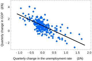
In statistics, linear regression is a statistical model which estimates the linear relationship between a scalar response and one or more explanatory variables. The case of one explanatory variable is called simple linear regression; for more than one, the process is called multiple linear regression. This term is distinct from multivariate linear regression, where multiple correlated dependent variables are predicted, rather than a single scalar variable. If the explanatory variables are measured with error then errors-in-variables models are required, also known as measurement error models.
In statistics, specifically regression analysis, a binary regression estimates a relationship between one or more explanatory variables and a single output binary variable. Generally the probability of the two alternatives is modeled, instead of simply outputting a single value, as in linear regression.

In statistics, a sequence of random variables is homoscedastic if all its random variables have the same finite variance; this is also known as homogeneity of variance. The complementary notion is called heteroscedasticity, also known as heterogeneity of variance. The spellings homoskedasticity and heteroskedasticity are also frequently used. Skedasticity comes from the Ancient Greek word skedánnymi, meaning “to scatter”. Assuming a variable is homoscedastic when in reality it is heteroscedastic results in unbiased but inefficient point estimates and in biased estimates of standard errors, and may result in overestimating the goodness of fit as measured by the Pearson coefficient.


