Arc length

Arc length is the distance between two points along a section of a curve. Development of a formulation of arc length suitable for applications to mathematics and the sciences is a focus of calculus. In the most basic formulation of arc length for a parametric curve (thought of as the trajectory of a particle), the arc length is gotten by integrating the speed of the particle over the path. Thus the length of a continuously differentiable curve ${\displaystyle (x(t),y(t))}$, for ${\displaystyle a\leq t\leq b}$, in the Euclidean plane is given as the integral $${\displaystyle L=\int _{a}^{b}{\sqrt {x'(t)^{2}+y'(t)^{2}}}\,dt,}$$ (because ${\displaystyle {\sqrt {x'(t)^{2}+y'(t)^{2}}}}$ is the magnitude of the velocity vector ${\displaystyle (x(t),y(t))}$, i.e., the particle's speed).

Contents

• General approach
• Formula for a smooth curve
• Finding arc lengths by integration
• Numerical integration
• Curve on a surface
• Other coordinate systems
• Simple cases
• Arcs of circles
• Other simple cases
• Historical methods
• Antiquity
• 17th century
• Integral form
• Curves with infinite length
• Generalization to (pseudo-)Riemannian manifolds
• See also
• References
• Sources
• External links

The defining integral of arc length does not always have a closed-form expression, and numerical integration may be used instead to obtain numerical values of arc length.

Determining the length of an irregular arc segment by approximating the arc segment as connected (straight) line segments is also called curve rectification. For a rectifiable curve these approximations don't get arbitrarily large (so the curve has a finite length).

General approach

A curve in the plane can be approximated by connecting a finite number of points on the curve using (straight) line segments to create a polygonal path. Since it is straightforward to calculate the length of each linear segment (using the Pythagorean theorem in Euclidean space, for example), the total length of the approximation can be found by summation of the lengths of each linear segment; that approximation is known as the (cumulative) chordal distance. ^[1]

If the curve is not already a polygonal path, then using a progressively larger number of line segments of smaller lengths will result in better curve length approximations. Such a curve length determination by approximating the curve as connected (straight) line segments is called rectification of a curve. The lengths of the successive approximations will not decrease and may keep increasing indefinitely, but for smooth curves they will tend to a finite limit as the lengths of the segments get arbitrarily small.

For some curves, there is a smallest number ${\displaystyle L}$ that is an upper bound on the length of all polygonal approximations (rectification). These curves are called rectifiable and the arc length is defined as the number ${\displaystyle L}$.

A signed arc length can be defined to convey a sense of orientation or "direction" with respect to a reference point taken as origin in the curve (see also: curve orientation and signed distance). ^[2]

Formula for a smooth curve

Let ${\displaystyle f\colon [a,b]\to \mathbb {R} ^{n}}$ be continuously differentiable (i.e., the derivative is a continuous function) function. The length of the curve is given by the formula $${\displaystyle L(f)=\int _{a}^{b}|f'(t)|\,dt}$$ where ${\displaystyle |f'(t)|}$ is the Euclidean norm of the tangent vector ${\displaystyle f'(t)}$ to the curve.

To justify this formula, define the arc length as limit of the sum of linear segment lengths for a regular partition of ${\displaystyle [a,b]}$ as the number of segments approaches infinity. This means

$${\displaystyle L(f)=\lim _{N\to \infty }\sum _{i=1}^{N}{\bigg |}f(t_{i})-f(t_{i-1}){\bigg |}}$$

where ${\displaystyle t_{i}=a+i(b-a)/N=a+i\Delta t}$ with ${\displaystyle \Delta t={\frac {b-a}{N}}=t_{i}-t_{i-1}}$ for ${\displaystyle i=0,1,\dotsc ,N.}$ This definition is equivalent to the standard definition of arc length as an integral:

$${\displaystyle L(f)=\lim _{N\to \infty }\sum _{i=1}^{N}{\bigg |}f(t_{i})-f(t_{i-1}){\bigg |}=\lim _{N\to \infty }\sum _{i=1}^{N}\left|{\frac {f(t_{i})-f(t_{i-1})}{\Delta t}}\right|\Delta t=\int _{a}^{b}{\Big |}f'(t){\Big |}\ dt.}$$

The last equality is proved by the following steps:

1. The second fundamental theorem of calculus shows $${\displaystyle f(t_{i})-f(t_{i-1})=\int _{t_{i-1}}^{t_{i}}f'(t)\ dt=\Delta t\int _{0}^{1}f'(t_{i-1}+\theta (t_{i}-t_{i-1}))\ d\theta }$$ where ${\displaystyle t=t_{i-1}+\theta (t_{i}-t_{i-1})}$ over ${\displaystyle \theta \in [0,1]}$ maps to ${\displaystyle [t_{i-1},t_{i}]}$ and ${\displaystyle dt=(t_{i}-t_{i-1})\,d\theta =\Delta t\,d\theta }$. In the below step, the following equivalent expression is used.$${\displaystyle {\frac {f(t_{i})-f(t_{i-1})}{\Delta t}}=\int _{0}^{1}f'(t_{i-1}+\theta (t_{i}-t_{i-1}))\ d\theta .}$$
2. The function ${\displaystyle \left|f'\right|}$ is a continuous function from a closed interval ${\displaystyle [a,b]}$ to the set of real numbers, thus it is uniformly continuous according to the Heine–Cantor theorem, so there is a positive real and monotonically non-decreasing function ${\displaystyle \delta (\varepsilon )}$ of positive real numbers ${\displaystyle \varepsilon }$ such that ${\displaystyle \Delta t<\delta (\varepsilon )}$ implies ${\displaystyle \left|\left|f'(t_{i-1}+\theta (t_{i}-t_{i-1}))\right|-\left|f'(t_{i})\right|\right|<\varepsilon }$ where ${\displaystyle \Delta t=t_{i}-t_{i-1}}$ and ${\displaystyle \theta \in [0,1]}$. Let's consider the limit ${\displaystyle {\ce {N\to \infty }}}$ of the following formula,$${\displaystyle \sum _{i=1}^{N}\left|{\frac {f(t_{i})-f(t_{i-1})}{\Delta t}}\right|\Delta t-\sum _{i=1}^{N}\left|f'(t_{i})\right|\Delta t.}$$

With the above step result, it becomes

$${\displaystyle \sum _{i=1}^{N}\left|\int _{0}^{1}f'(t_{i-1}+\theta (t_{i}-t_{i-1}))\ d\theta \right|\Delta t-\sum _{i=1}^{N}\left|f'(t_{i})\right|\Delta t.}$$

Terms are rearranged so that it becomes

$${\displaystyle {\begin{aligned}&\Delta t\sum _{i=1}^{N}\left(\left|\int _{0}^{1}f'(t_{i-1}+\theta (t_{i}-t_{i-1}))\ d\theta \right|-\int _{0}^{1}\left|f'(t_{i})\right|d\theta \right)\\&\qquad \leqq \Delta t\sum _{i=1}^{N}\left(\int _{0}^{1}\left|f'(t_{i-1}+\theta (t_{i}-t_{i-1}))\right|\ d\theta -\int _{0}^{1}\left|f'(t_{i})\right|d\theta \right)\\&\qquad =\Delta t\sum _{i=1}^{N}\int _{0}^{1}\left|f'(t_{i-1}+\theta (t_{i}-t_{i-1}))\right|-\left|f'(t_{i})\right|\ d\theta \end{aligned}}}$$

where in the leftmost side ${\textstyle \left|f'(t_{i})\right|=\int _{0}^{1}\left|f'(t_{i})\right|d\theta }$ is used. By ${\textstyle \left|\left|f'(t_{i-1}+\theta (t_{i}-t_{i-1}))\right|-\left|f'(t_{i})\right|\right|<\varepsilon }$ for ${\textstyle N>(b-a)/\delta (\varepsilon )}$ so that ${\displaystyle \Delta t<\delta (\varepsilon )}$, it becomes

$${\displaystyle \Delta t\sum _{i=1}^{N}\left(\left|\int _{0}^{1}f'(t_{i-1}+\theta (t_{i}-t_{i-1}))\ d\theta \right|-\left|f'(t_{i})\right|\right)<\varepsilon N\Delta t}$$

with ${\displaystyle \left|f'(t_{i})\right|=\int _{0}^{1}\left|f'(t_{i})\right|d\theta }$, ${\displaystyle \varepsilon N\Delta t=\varepsilon (b-a)}$, and ${\displaystyle N>(b-a)/\delta (\varepsilon )}$. In the limit ${\displaystyle N\to \infty ,}$${\displaystyle \delta (\varepsilon )\to 0}$ so ${\displaystyle \varepsilon \to 0}$ thus the left side of ${\displaystyle <}$ approaches ${\displaystyle 0}$. In other words, ${\displaystyle \sum _{i=1}^{N}\left|{\frac {f(t_{i})-f(t_{i-1})}{\Delta t}}\right|\Delta t=\sum _{i=1}^{N}\left|f'(t_{i})\right|\Delta t}$ in this limit, and the right side of this equality is just the Riemann integral of ${\displaystyle \left|f'(t)\right|}$ on ${\displaystyle [a,b].}$ This definition of arc length shows that the length of a curve represented by a continuously differentiable function ${\displaystyle f:[a,b]\to \mathbb {R} ^{n}}$ on ${\displaystyle [a,b]}$ is always finite, i.e., rectifiable.

The definition of arc length of a smooth curve as the integral of the norm of the derivative is equivalent to the definition

$${\displaystyle L(f)=\sup \sum _{i=1}^{N}{\bigg |}f(t_{i})-f(t_{i-1}){\bigg |}}$$

where the supremum is taken over all possible partitions ${\displaystyle a=t_{0}<t_{1}<\dots <t_{N-1}<t_{N}=b}$ of ${\displaystyle [a,b].}$ ^[3] This definition as the supremum of the all possible partition sums is also valid if ${\displaystyle f}$ is merely continuous, not differentiable.

A curve can be parameterized in infinitely many ways. Let ${\displaystyle \varphi$ :[a,b]\to [c,d]} be any continuously differentiable bijection. Then ${\displaystyle g=f\circ \varphi ^{-1}:[c,d]\to \mathbb {R} ^{n}}$ is another continuously differentiable parameterization of the curve originally defined by ${\displaystyle f.}$ The arc length of the curve is the same regardless of the parameterization used to define the curve:

$${\displaystyle {\begin{aligned}L(f)&=\int _{a}^{b}{\Big |}f'(t){\Big |}\ dt=\int _{a}^{b}{\Big |}g'(\varphi (t))\varphi '(t){\Big |}\ dt\\&=\int _{a}^{b}{\Big |}g'(\varphi (t)){\Big |}\varphi '(t)\ dt\quad {\text{in the case }}\varphi {\text{ is non-decreasing}}\\&=\int _{c}^{d}{\Big |}g'(u){\Big |}\ du\quad {\text{using integration by substitution}}\\&=L(g).\end{aligned}}}$$

Finding arc lengths by integration

If a planar curve in ${\displaystyle \mathbb {R} ^{2}}$ is defined by the equation ${\displaystyle y=f(x),}$ where ${\displaystyle f}$ is continuously differentiable, then it is simply a special case of a parametric equation where ${\displaystyle x=t}$ and ${\displaystyle y=f(t).}$ The Euclidean distance of each infinitesimal segment of the arc can be given by:

$${\displaystyle {\sqrt {dx^{2}+dy^{2}}}={\sqrt {1+\left({\frac {dy}{dx}}\right)^{2}\,}}dx.}$$

The arc length is then given by:

$${\displaystyle s=\int _{a}^{b}{\sqrt {1+\left({\frac {dy}{dx}}\right)^{2}\,}}dx.}$$

Curves with closed-form solutions for arc length include the catenary, circle, cycloid, logarithmic spiral, parabola, semicubical parabola and straight line. The lack of a closed form solution for the arc length of an elliptic and hyperbolic arc led to the development of the elliptic integrals.

Simple cases

Historical methods

Integral form

Before the full formal development of calculus, the basis for the modern integral form for arc length was independently discovered by Hendrik van Heuraet and Pierre de Fermat.

In 1659 van Heuraet published a construction showing that the problem of determining arc length could be transformed into the problem of determining the area under a curve (i.e., an integral). As an example of his method, he determined the arc length of a semicubical parabola, which required finding the area under a parabola. ^[9] In 1660, Fermat published a more general theory containing the same result in his De linearum curvarum cum lineis rectis comparatione dissertatio geometrica (Geometric dissertation on curved lines in comparison with straight lines). ^[10]

Building on his previous work with tangents, Fermat used the curve

${\displaystyle y=x^{\frac {3}{2}}\,}$

whose tangent at x = a had a slope of

${\displaystyle {3 \over 2}a^{\frac {1}{2}}}$

so the tangent line would have the equation

${\displaystyle y={3 \over 2}a^{\frac {1}{2}}(x-a)+f(a).}$

Next, he increased a by a small amount to a + ε, making segment AC a relatively good approximation for the length of the curve from A to D. To find the length of the segment AC, he used the Pythagorean theorem:

${\displaystyle {\begin{aligned}AC^{2}&=AB^{2}+BC^{2}\\&=\varepsilon ^{2}+{9 \over 4}a\varepsilon ^{2}\\&=\varepsilon ^{2}\left(1+{9 \over 4}a\right)\end{aligned}}}$

which, when solved, yields

${\displaystyle AC=\varepsilon {\sqrt {1+{9 \over 4}a\,}}.}$

In order to approximate the length, Fermat would sum up a sequence of short segments.

Curves with infinite length

As mentioned above, some curves are non-rectifiable. That is, there is no upper bound on the lengths of polygonal approximations; the length can be made arbitrarily large. Informally, such curves are said to have infinite length. There are continuous curves on which every arc (other than a single-point arc) has infinite length. An example of such a curve is the Koch curve. Another example of a curve with infinite length is the graph of the function defined by f(x) = x sin(1/x) for any open set with 0 as one of its delimiters and f(0) = 0. Sometimes the Hausdorff dimension and Hausdorff measure are used to quantify the size of such curves.

Generalization to (pseudo-)Riemannian manifolds

Let ${\displaystyle M}$ be a (pseudo-)Riemannian manifold, ${\displaystyle g}$ the (pseudo-) metric tensor, ${\displaystyle \gamma$ :[0,1]\rightarrow M} a curve in ${\displaystyle M}$ defined by ${\displaystyle n}$ parametric equations

${\displaystyle \gamma (t)=[\gamma ^{1}(t),\dots ,\gamma ^{n}(t)],\quad t\in [0,1]}$

and

${\displaystyle \gamma (0)=\mathbf {x} ,\,\,\gamma (1)=\mathbf {y} }$

The length of ${\displaystyle \gamma }$, is defined to be

${\displaystyle \ell (\gamma )=\int \limits _{0}^{1}||\gamma '(t)||_{\gamma (t)}dt}$,

or, choosing local coordinates ${\displaystyle x}$,

${\displaystyle \ell (\gamma )=\int \limits _{0}^{1}{\sqrt {\pm \sum _{i,j=1}^{n}g_{ij}(x(\gamma (t))){\frac {dx^{i}(\gamma (t))}{dt}}{\frac {dx^{j}(\gamma (t))}{dt}}}}dt}$,

where

${\displaystyle \gamma '(t)\in T_{\gamma (t)}M}$

is the tangent vector of ${\displaystyle \gamma }$ at ${\displaystyle t.}$ The sign in the square root is chosen once for a given curve, to ensure that the square root is a real number. The positive sign is chosen for spacelike curves; in a pseudo-Riemannian manifold, the negative sign may be chosen for timelike curves. Thus the length of a curve is a non-negative real number. Usually no curves are considered which are partly spacelike and partly timelike.

In theory of relativity, arc length of timelike curves (world lines) is the proper time elapsed along the world line, and arc length of a spacelike curve the proper distance along the curve.

See also

• Arc (geometry)
• Circumference
• Crofton formula
• Elliptic integral
• Geodesics
• Intrinsic equation
• Integral approximations
• Line integral
• Meridian arc
• Multivariable calculus
• Sinuosity

Related Research Articles

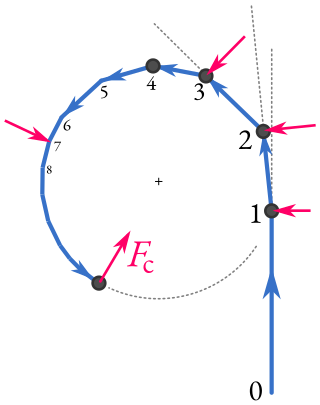
A centripetal force is a force that makes a body follow a curved path. The direction of the centripetal force is always orthogonal to the motion of the body and towards the fixed point of the instantaneous center of curvature of the path. Isaac Newton described it as "a force by which bodies are drawn or impelled, or in any way tend, towards a point as to a centre". In Newtonian mechanics, gravity provides the centripetal force causing astronomical orbits.

In mathematics, the polar coordinate system is a two-dimensional coordinate system in which each point on a plane is determined by a distance from a reference point and an angle from a reference direction. The reference point is called the pole, and the ray from the pole in the reference direction is the polar axis. The distance from the pole is called the radial coordinate, radial distance or simply radius, and the angle is called the angular coordinate, polar angle, or azimuth. Angles in polar notation are generally expressed in either degrees or radians.

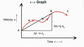
In physics, equations of motion are equations that describe the behavior of a physical system in terms of its motion as a function of time. More specifically, the equations of motion describe the behavior of a physical system as a set of mathematical functions in terms of dynamic variables. These variables are usually spatial coordinates and time, but may include momentum components. The most general choice are generalized coordinates which can be any convenient variables characteristic of the physical system. The functions are defined in a Euclidean space in classical mechanics, but are replaced by curved spaces in relativity. If the dynamics of a system is known, the equations are the solutions for the differential equations describing the motion of the dynamics.

In science, work is the energy transferred to or from an object via the application of force along a displacement. In its simplest form, for a constant force aligned with the direction of motion, the work equals the product of the force strength and the distance traveled. A force is said to do positive work if it has a component in the direction of the displacement of the point of application. A force does negative work if it has a component opposite to the direction of the displacement at the point of application of the force.

In mathematics, the Laplace operator or Laplacian is a differential operator given by the divergence of the gradient of a scalar function on Euclidean space. It is usually denoted by the symbols , (where is the nabla operator), or . In a Cartesian coordinate system, the Laplacian is given by the sum of second partial derivatives of the function with respect to each independent variable. In other coordinate systems, such as cylindrical and spherical coordinates, the Laplacian also has a useful form. Informally, the Laplacian Δf (p) of a function f at a point p measures by how much the average value of f over small spheres or balls centered at p deviates from f (p).

In continuum mechanics, the infinitesimal strain theory is a mathematical approach to the description of the deformation of a solid body in which the displacements of the material particles are assumed to be much smaller than any relevant dimension of the body; so that its geometry and the constitutive properties of the material at each point of space can be assumed to be unchanged by the deformation.

In the mathematical field of differential geometry, a metric tensor is an additional structure on a manifold M that allows defining distances and angles, just as the inner product on a Euclidean space allows defining distances and angles there. More precisely, a metric tensor at a point p of M is a bilinear form defined on the tangent space at p, and a metric field on M consists of a metric tensor at each point p of M that varies smoothly with p.

In geometry, a solid of revolution is a solid figure obtained by rotating a plane figure around some straight line, which may not intersect the generatrix. The surface created by this revolution and which bounds the solid is the surface of revolution.

A surface of revolution is a surface in Euclidean space created by rotating a curve one full revolution around an axis of rotation . The volume bounded by the surface created by this revolution is the solid of revolution.

In analytical mechanics, generalized coordinates are a set of parameters used to represent the state of a system in a configuration space. These parameters must uniquely define the configuration of the system relative to a reference state. The generalized velocities are the time derivatives of the generalized coordinates of the system. The adjective "generalized" distinguishes these parameters from the traditional use of the term "coordinate" to refer to Cartesian coordinates.

In information geometry, the Fisher information metric is a particular Riemannian metric which can be defined on a smooth statistical manifold, i.e., a smooth manifold whose points are probability measures defined on a common probability space. It can be used to calculate the informational difference between measurements.

In geometry, the line element or length element can be informally thought of as a line segment associated with an infinitesimal displacement vector in a metric space. The length of the line element, which may be thought of as a differential arc length, is a function of the metric tensor and is denoted by .

In geometry, an envelope of a planar family of curves is a curve that is tangent to each member of the family at some point, and these points of tangency together form the whole envelope. Classically, a point on the envelope can be thought of as the intersection of two "infinitesimally adjacent" curves, meaning the limit of intersections of nearby curves. This idea can be generalized to an envelope of surfaces in space, and so on to higher dimensions.

In mechanics, virtual work arises in the application of the principle of least action to the study of forces and movement of a mechanical system. The work of a force acting on a particle as it moves along a displacement is different for different displacements. Among all the possible displacements that a particle may follow, called virtual displacements, one will minimize the action. This displacement is therefore the displacement followed by the particle according to the principle of least action.

The work of a force on a particle along a virtual displacement is known as the virtual work.

An osculating circle is a circle that best approximates the curvature of a curve at a specific point. It is tangent to the curve at that point and has the same curvature as the curve at that point. The osculating circle provides a way to understand the local behavior of a curve and is commonly used in differential geometry and calculus.

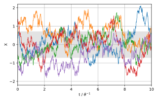
In mathematics, the Ornstein–Uhlenbeck process is a stochastic process with applications in financial mathematics and the physical sciences. Its original application in physics was as a model for the velocity of a massive Brownian particle under the influence of friction. It is named after Leonard Ornstein and George Eugene Uhlenbeck.

In calculus, the Leibniz integral rule for differentiation under the integral sign, named after Gottfried Wilhelm Leibniz, states that for an integral of the form where and the integrands are functions dependent on the derivative of this integral is expressible as where the partial derivative indicates that inside the integral, only the variation of with is considered in taking the derivative.

A pendulum is a body suspended from a fixed support such that it freely swings back and forth under the influence of gravity. When a pendulum is displaced sideways from its resting, equilibrium position, it is subject to a restoring force due to gravity that will accelerate it back towards the equilibrium position. When released, the restoring force acting on the pendulum's mass causes it to oscillate about the equilibrium position, swinging it back and forth. The mathematics of pendulums are in general quite complicated. Simplifying assumptions can be made, which in the case of a simple pendulum allow the equations of motion to be solved analytically for small-angle oscillations.

In mathematics, vector spherical harmonics (VSH) are an extension of the scalar spherical harmonics for use with vector fields. The components of the VSH are complex-valued functions expressed in the spherical coordinate basis vectors.

In mathematics, a line integral is an integral where the function to be integrated is evaluated along a curve. The terms path integral, curve integral, and curvilinear integral are also used; contour integral is used as well, although that is typically reserved for line integrals in the complex plane.

References

Sources

• Farouki, Rida T. (1999). "Curves from motion, motion from curves". In Laurent, P.-J.; Sablonniere, P.; Schumaker, L. L. (eds.). Curve and Surface Design: Saint-Malo 1999. Vanderbilt Univ. Press. pp. 63–90. ISBN   978-0-8265-1356-4.

External links

Wikimedia Commons has media related to Arc length .

• "Rectifiable curve", Encyclopedia of Mathematics , EMS Press, 2001 [1994]
• The History of Curvature
• Weisstein, Eric W. "Arc Length". MathWorld .
• Arc Length by Ed Pegg Jr., The Wolfram Demonstrations Project, 2007.
• Calculus Study Guide – Arc Length (Rectification)
• Famous Curves Index The MacTutor History of Mathematics archive
• Arc Length Approximation by Chad Pierson, Josh Fritz, and Angela Sharp, The Wolfram Demonstrations Project.
• Length of a Curve Experiment Illustrates numerical solution of finding length of a curve.