Image Texture Analysis
- 1. Image Texture Analysis Lalit Gupta, Scientist, Philips Research
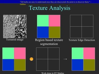
- 2. Texture Analysis Region based texture segmentation Textured image + Texture Edge Detection
- 3. Region Based Texture Segmentation
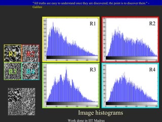
- 4. Image histograms R1 R2 R3 R4 R1 R2 R3 R4
- 5. Classification using Proposed Methodology Image DWT: Discrete wavelet transform DCT: Discrete cosine transform Ref: [Randen99] A1 V1 H1 D1 1 ST level Decomposition DWT (Daubechies) D j D j Filtering FCM Unsupervised classification DCT (9 masks) DCT (9 masks) . . Gaussian filtering G j G j Smoothing . . Mean F j F j Feature extraction . .
- 6. Input Image Steps of Processing DWT A1 V1 H1 D1 FCM .. .. .. DCT . . . .. .. .. Smoothing . . . .. .. .. Mean 36 Feature images . . .
- 7. Results using various Filtering Techniques (a) Input Image Ref: [Ng92], [Rao2004], [Cesmeli2001] (b) DWT (c) Gabor filter (b) DWT+Gabor (d) GMRF (e) DWT + MRF (f) DCT (f) DWT+DCT
- 8. Results (Cont.) I1 I2 I3 I4 I5 Input images I6 I7 I8 I9 I10
- 11. Proposed Methodology Input image Ref: [Liu99], [Canny86], [Yegnanarayana98] Filtering using 1-D Discrete Wavelet Transform and 1-D Gabor filter bank 16 dimensional feature vector is mapped onto one dimensional feature map Self-Organizing feature Map (SOM) Smoothed image Smoothing using 2-D symmetric Gaussian filter Edge map Edge detection using Canny operator Final edge map Edge Linking Smoothed images Smoothing using 2-D asymmetric Gaussian filter . . . 16 filtered images, 8 each along horizontal and vertical parallel lines of image . . .
- 12. Steps of Processing Input image Filtered images ... ... Smoothed images Feature map Smoothed images Edge map
- 13. Results Input image Edge map Input image Edge map Input image Edge map
- 14. Integrating Region and Edge Information for Texture Segmentation We have used a modified constraint satisfaction neural networks termed as Constraint Satisfaction Neural Network for Complementary Information Integration (CSNN-CII), which integrates the region and edge based approaches. +
- 15. Dynamic Window Image Window
- 16. Constraint Satisfaction Neural Networks For Image Segmentation 1 < i < n 1 < j < n 1 < k < m Size of image: n x n No. of labels/classes: m Ref: [Lin92] i j k
- 17. Constraint Satisfaction Neural Network for Complementary Information Integration (CSNN-CII) Each neuron in CSNN-CII contains two fields: Probability and Rank. Probability: probability that the pixel belongs to the segment represented by the corresponding layer. Rank: Rank field stores the rank of the probability in a decreasing order, for that neuron. 0.1 0.5 0.4 Probabilities 3 1 2 Rank
- 18. The weight between k th layer’s ( i, j ) th , U ijk , neuron and l th layer’s ( q, r ) th , U qrl , neuron is computed as: Weights in the CSNN can be interpreted as constraints. Weights are determined based on the heuristic that a neuron excites other neurons representing the labels of similar intensities and inhibits other neurons representing labels of quite different intensities. Where, p : number of neurons in 2D neighborhood (dynamic window). m : number of layers (classes). U ijk : represents k th layer’s ( i , j ) th neuron. R ijk : Rank for ( i, j ) th neuron in k th layer or U ijk neuron. Ref: [Lin 92] U ijk U qrl W ij,qr,k,l
- 19. Algorithm Phase 1: Initialize the CSNN neurons using fuzzy c-means results. The probability values obtained from FCM are assigned to the nodes of CSNN. Ranks for each neuron are also computed on the basis of initial class probabilities. FCM output 0.2 0.2 0.8 0.3 0.6 0.2 0.6 0.3 0.6 0.8 0.8 0.2 0.7 0.4 0.8 0.4 0.7 0.4 0.2, 2 0.2, 2 0.8, 1 0.3, 2 0.6, 1 0.2, 2 0.6, 1 0.3, 2 0.6, 1 0.8, 1 0.8, 1 0.2, 2 0.7, 1 0.4, 2 0.8, 1 0.4, 2 0.7, 1 0.4, 2 Rank Probability CSNN-CII Layer-1 Layer-2
- 20. H ijk : sum of inputs from all neighboring neurons. O ijk : the probability of ( i , j ) th pixel having a label k (Probability value assigned to the U ijk neuron) . N ij : a set of neurons in the 3D neighborhood of ( i,j ) th neuron (considering Dynamic window). Iterate and update the probabilities, edge map and determine the winner label Algorithm (Cont.) U ijk H ijk i j k
- 21. CSNN-CII Layer-1 Layer-2 Algorithm (Cont.) Edge information 0.2, 2 0.2, 2 0.8, 1 0.3, 2 0.6, 1 0.2, 2 0.6, 1 0.3, 2 0.6, 1 0.8, 1 0.8, 1 0.2, 2 0.7, 1 0.4, 2 0.8, 1 0.4, 2 0.7, 1 0.4, 2 For neurons with rank=1 For neurons with rank=2 1 0 0 1 0 0 1 0 0
- 22. Algorithm (Cont.) CSNN-CII Layer-1 Layer-2 0.2, 2 0.2, 2 0.8, 1 0.3, 2 0.6, 1 0.2, 2 0.6, 1 0.3, 2 0.6, 1 0.8, 1 0.8, 1 0.2, 2 0.7, 1 0.4, 2 0.8, 1 0.4, 2 0.7, 1 0.4, 2
- 23. Where, Algorithm (Cont.) Labels to each pixel of an image are assigned as: Where, l l m Updated probability values: 0.2, 2 0.2, 2 0.8, 1 0.3, 2 0.6, 1 0.2, 2 0.6, 1 0.3, 2 0.6, 1 0.8, 1 0.8, 1 0.2, 2 0.7, 1 0.4, 2 0.8, 1 0.4, 2 0.7, 1 0.4, 2 2 2 1 2 1 2 1 2 1 Layer-1 Layer-2 Y
- 24. Updating Edge Map: B : Edge map obtained using lower threshold. E : Edge map obtained using higher threshold. M ij : the set of pixels in the neighborhood of pixel ( i , j ) in the output image Y of size 2 v+ 1 , excluding edge pixels in E. Algorithm (Cont.) Y E Edge map at each iteration is computed as:
- 25. Check the convergence condition, i.e., the number of pixels updated in Y , at each iteration. If there is any update go to second step. Algorithm (Cont.) Edge map at each iteration is computed as: B Y Updated edge map ( E ) E M
- 26. Phase 2 Iterate, and update edge map E, by removing extra edge pixels and by adding new edge pixels. Algorithm (Cont.) L ij is considered as: Edge map E is updated as: Y
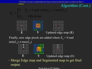
- 27. Merge Edge map and Segmented map to get final output. Finally, new edge pixels are added where E ij = 0 and min( L ij ) max( L ij ) Algorithm (Cont.) E Y Updated edge map ( E ) E Y Updated edge map (E)
- 28. Merge Edge map and Segmented map to get final output. Final Output Segmented map Edge map
- 29. Input Image Segmented map before integration ( Ref: [Rao2004] ) Edge map before integration ( Ref: [Lalit2006] ) Segmented map and Edge map after integration Results
- 30. Results Input Image Segmented map before integration ( Ref: [Rao2004] ) Edge map before integration ( Ref: [Lalit2006] ) Segmented map and Edge map after integration


![Classification using Proposed Methodology Image DWT: Discrete wavelet transform DCT: Discrete cosine transform Ref: [Randen99] A1 V1 H1 D1 1 ST level Decomposition DWT (Daubechies) D j D j Filtering FCM Unsupervised classification DCT (9 masks) DCT (9 masks) . . Gaussian filtering G j G j Smoothing . . Mean F j F j Feature extraction . .](https://image.slidesharecdn.com/imagetextureanalysis-1291267252153-phpapp01/85/Image-Texture-Analysis-5-320.jpg)

![Results using various Filtering Techniques (a) Input Image Ref: [Ng92], [Rao2004], [Cesmeli2001] (b) DWT (c) Gabor filter (b) DWT+Gabor (d) GMRF (e) DWT + MRF (f) DCT (f) DWT+DCT](https://image.slidesharecdn.com/imagetextureanalysis-1291267252153-phpapp01/85/Image-Texture-Analysis-7-320.jpg)


![Proposed Methodology Input image Ref: [Liu99], [Canny86], [Yegnanarayana98] Filtering using 1-D Discrete Wavelet Transform and 1-D Gabor filter bank 16 dimensional feature vector is mapped onto one dimensional feature map Self-Organizing feature Map (SOM) Smoothed image Smoothing using 2-D symmetric Gaussian filter Edge map Edge detection using Canny operator Final edge map Edge Linking Smoothed images Smoothing using 2-D asymmetric Gaussian filter . . . 16 filtered images, 8 each along horizontal and vertical parallel lines of image . . .](https://image.slidesharecdn.com/imagetextureanalysis-1291267252153-phpapp01/85/Image-Texture-Analysis-11-320.jpg)


![Constraint Satisfaction Neural Networks For Image Segmentation 1 < i < n 1 < j < n 1 < k < m Size of image: n x n No. of labels/classes: m Ref: [Lin92] i j k](https://image.slidesharecdn.com/imagetextureanalysis-1291267252153-phpapp01/85/Image-Texture-Analysis-16-320.jpg)

![The weight between k th layer’s ( i, j ) th , U ijk , neuron and l th layer’s ( q, r ) th , U qrl , neuron is computed as: Weights in the CSNN can be interpreted as constraints. Weights are determined based on the heuristic that a neuron excites other neurons representing the labels of similar intensities and inhibits other neurons representing labels of quite different intensities. Where, p : number of neurons in 2D neighborhood (dynamic window). m : number of layers (classes). U ijk : represents k th layer’s ( i , j ) th neuron. R ijk : Rank for ( i, j ) th neuron in k th layer or U ijk neuron. Ref: [Lin 92] U ijk U qrl W ij,qr,k,l](https://image.slidesharecdn.com/imagetextureanalysis-1291267252153-phpapp01/85/Image-Texture-Analysis-18-320.jpg)



![Input Image Segmented map before integration ( Ref: [Rao2004] ) Edge map before integration ( Ref: [Lalit2006] ) Segmented map and Edge map after integration Results](https://image.slidesharecdn.com/imagetextureanalysis-1291267252153-phpapp01/85/Image-Texture-Analysis-29-320.jpg)
![Results Input Image Segmented map before integration ( Ref: [Rao2004] ) Edge map before integration ( Ref: [Lalit2006] ) Segmented map and Edge map after integration](https://image.slidesharecdn.com/imagetextureanalysis-1291267252153-phpapp01/85/Image-Texture-Analysis-30-320.jpg)