The drop-down list is a powerful feature in Excel that allows users to select values from predefined options instead of manual typing, providing better data entry accuracy and efficiency. Whether you are a beginner or an experienced Excel user, understanding and utilizing drop-down lists can greatly enhance your productivity and data management capabilities. In this article, we will step-by-step introduce different ways to create a drop-down list in Excel.

• Create a drop-down list
• By manually input
• From a range
• By Kutools with fewer clicks
• From a table (dynamic)
• From a range name
• From another workbook
• Error Alert (allow other entries)
• Input Message
• Other notes

---

Video: Create a drop down list

Create a drop-down list

Let's start to learn how to create a drop-down list in Excel.

Create a drop-down list by manually input

Step 1: Select the cell(s) that you want to place the drop-down list

Step 2: Go to click Data tab, and click Data Validation

Step 3: Specify settings in the Data Validation dialog

Under Settings tab, please specify below settings:

1. Choose List from Allow drop-down list;
2. Type the items that you want to display in the drop-down list in the Source section, separate them by a comma;
3. Click OK.

Result:

Now the drop-down list has been created.

Create a drop-down list from a range

To create a drop-down list based on a range of cell values, please follow below steps:

Step 1: Select the cell(s) that you want to place the drop-down list

Step 2: Go to click Data tab, and click Data Validation

Step 3: Specify settings in the Data Validation dialog

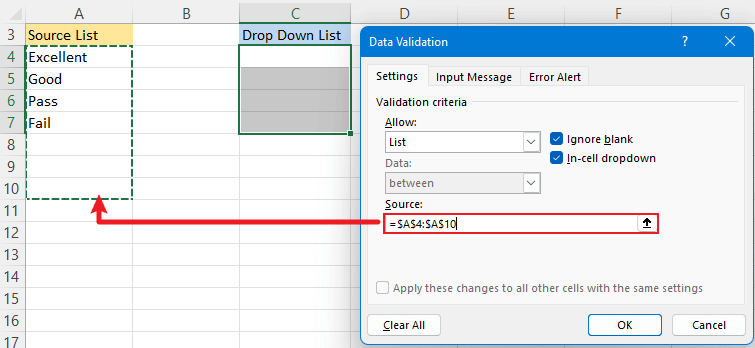
Under Settings tab, please specify below settings:

1. Choose List from Allow drop-down list;
2. Click selection icon to select the source list in the Source section;
3. Click OK.

Result:

Now the drop-down list has been created.

Create a drop-down list with Kutools

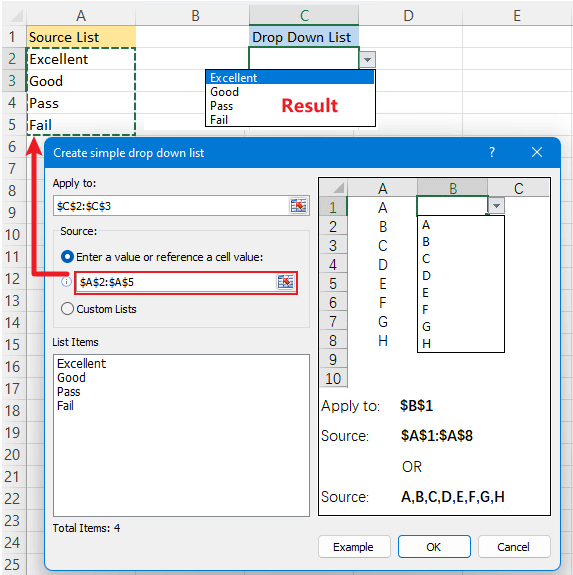
Here is a handy feature – Create simple drop-down list of Kutools for Excel can let you quickly and easily create a drop-down list with fewer clicks. Here is how to do:

1. Select cell(s) to place the drop-down list;
2. Click Kutools tab, and click Drop-down List > Create simple drop down list;
3. Select the range of cells (or directly type items separated by a comma) that you want to show in the drop down list, click OK.
   

Create a drop-down list from a table (dynamic)

If you want to create a dynamic expandable drop-down list that updates automatically as you add or remove items from the source list, you should place the source data into an Excel table.

Step 1: Convert the source list to a table

Select the source list and click Insert > Table, and in the Create Table dialog, if the selection includes column header, please tick My table has headers, then click OK.

Step 2: Select the cell(s) that you want to place the drop-down list

Step 3: Go to click Data tab, and click Data Validation

Step 4: Specify settings in the Data Validation dialog

Under Settings tab, please specify below settings:

1. Choose List from Allow drop-down list;
2. Click selection icon to select the table range (excluding header) in the Source section;
3. Click OK.

Result:

The drop-down list has been created.

And when you add or remove items from the source table, the drop-down list will be updated at the same time.

Create a drop-down list from a range name

If you will create drop-down lists in multiple sheets based on a same source list, I recommend you to create a range name for the source list for easily referenced to.

Step 1: Create a range name for the source list

Select the source list and go to the name box (beside the formula bar), and type a name for it (the name cannot contain space or other special characters), then press Enter key to finish.

Step 2: Select the cell(s) that you want to place the drop-down list

Step 3: Go to click Data tab, and click Data Validation

Step 4: Specify settings in the Data Validation dialog

Under Settings tab, please specify below settings:

1. Choose List from Allow drop-down list;
2. Type an equal sign and followed by the name you set in step 1 in the Source section like

   =SourceList

   You can also click on the Source texbox and press F3 key to open Paste Name dialog, then choose the range name you want from the list, click OK to insert it to the textbox.
3. Click OK.

Result:

The drop-down list has been created.

Create a drop-down list from another workbook

If the source list and the to-be-created drop-down list are in different workbooks, when you select the source list in the Source section of Data Validation dialog, an alert will pop out to prevent the creation.

Here this part will tell you how to create a drop-down list from another workbook.

Step 1: Create a range name for the source list in source workbook

In the source workbook, select the source items that you want them appear in the drop-down list. Then go to the Name Box which is next to the Formula Bar, type a name, such as "SourceList".

Step 2: Define a name that references your source list in the drop-down list workbook

1. Enable the workbook where you want to create a drop-down list, click Formula > Define Name.

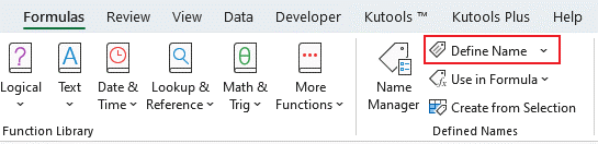   Define Name "/>

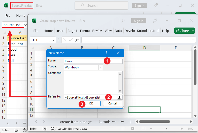
2. In the popping New Name dialog, set as below:

   1. Type a name in the Name box, such as Items;
   2. Type an equal sign followed by the source workbook name and the name you defined for the source list in step 1 in the Refers to box, such as

      =SourceFile.xlsx!SourceList

   3. Click OK.

       

Step 3: Select the cell(s) that you want to place the drop-down list

Step 4: Go to click Data tab, and click Data Validation

Step 5: Specify settings in the Data Validation dialog

Under Settings tab, please specify below settings:

1. Choose List from Allow drop-down list;
2. Type an equal sign followed by the name you defined in step 3 in the Source section, like

   =Items

3. Click OK.

   

Result:

The drop-down list has been created.

Error Alert (allow other entries)

By default, the drop-down list only allows values contained in the list to be entered into a cell. When you enter a value that does not exist in the drop-down list and press the Enter key, an error alert will show up, as shown in the screenshot below. When you click the Retry button, the entered value is selected for re-editing. Clicking the Cancel button will clear the entered value.

• If you want to allow users to type other values and stop the error alert showing, you can do as these:

  1. Select the drop-down list cells that you want to stop the error alert, click Data > Data Validation.

  2. In the Data Validation dialog, under Error Alert tab, untick the Show error alert after invalid data is entered checkbox. Click OK.

     

  Now when users type other values, there is no error alert showing up.

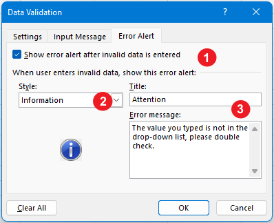
• If you want to allow users to type other values but also show an alert for reminding them, please do as these:

  1. Select the drop-down list cells that you want other values typed in, click Data > Data Validation.

  2. In the Data Validation dialog, under Error Alert tab:
     1. Keep the Show error alert after invalid data is entered checkbox ticked;
     2. Select Information from Style drop-down list;
     3. Specify the Title and Error message, click OK.

     

  From now on, when users type other values, a dialog pops out to remind, click OK to remain the typed value, click Cancel to clear the entered value.

  

Input Message

When creating a drop-down list, you can add an input message to remind users to select items from the drop-down list when selecting a cell, or other information you want to show.

1. Select the drop-down list cells that you want to add an input message, click Data > Data Validation.

2. In the Data Validation dialog, under Input Message tab

1. Keep the Show input message when cell is selected checkbox ticked;
2. Specify the Title and Input message, click OK.

Now, when users select the cell of drop-down list, a yellow textbox with information you provided shows up.

Other notes

1. By default, when a drop-down list is created, the "Ignore blank" checkbox is selected. This means that users can leave the cells blank without an alert popping.

   If the "Ignore blank" checkbox is unticked, the blank cells in the range will be treaed as invalid entries, the alert will pop out.

2. If you want to change the order of the items in the drop-down list, you could rearrange the source list.

3. If the Data Validation feature is disabled, it is possible that you are working in a protected worksheet. To enable Data Validation, simply unprotect the worksheet and then apply the desired Data Validation settings.