Linear transformation.ppt

Chapter 4 Linear TransformationsChapter 4 Linear Transformations
4.1 Introduction to Linear Transformations4.1 Introduction to Linear Transformations
4.2 The Kernel and Range of a Linear Transformation4.2 The Kernel and Range of a Linear Transformation
4.3 Matrices for Linear Transformations4.3 Matrices for Linear Transformations
4.4 Transition Matrices and Similarity4.4 Transition Matrices and Similarity

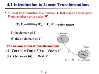
6 - 2
4.1 Introduction to Linear Transformations4.1 Introduction to Linear Transformations

A linear transformation is a function TT that maps a vector space
VV into another vector space WW:
mapping
: , , : vector spaceT V W V W→
V: the domain of T
W: the co-domain of T
(1) (u v) (u) (v), u, vT T T V+ = + ∀ ∈
(2) ( u) (u),T c cT c R= ∀ ∈
Two axioms of linear transformationsTwo axioms of linear transformations

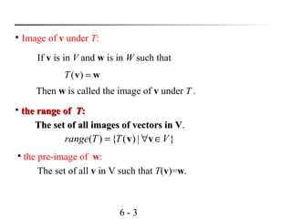
6 - 3

Image of v under T:
If v is in V and w is in W such that
wv =)(T
Then w is called the image of v under T .

the range ofthe range of TT::
The set of all images of vectors in VThe set of all images of vectors in V.

the pre-image of w:
The set of all v in V such that T(v)=w.
}|)({)( VTTrange ∈∀= vv

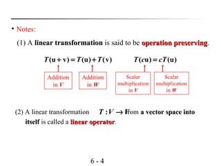
6 - 4

Notes:
(1) A linear transformationlinear transformation is said to be operation preservingoperation preserving.
(u v) (u) (v)T T T+ = +
Addition
in V
Addition
in W
( u) (u)T c cT=
Scalar
multiplication
in V
Scalar
multiplication
in W
(2) A linear transformation from a vector space intoa vector space into
itselfitself is called a linear operatorlinear operator.
:T V V→

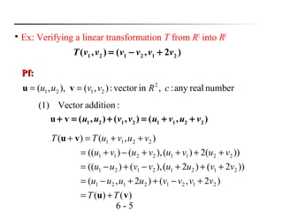
6 - 5

Ex: Verifying a linear transformation T from R2
into R2
Pf:Pf:
1 2 1 2 1 2( , ) ( , 2 )T v v v v v v= − +
numberrealany:,invector:),(),,( 2
2121 cRvvuu == vu
(1) Vector addition :
1 2 1 2 1 1 2 2u v ( , ) ( , ) ( , )u u v v u v u v+ = + = + +
)()(
)2,()2,(
))2()2(),()((
))(2)(),()((
),()(
21212121
21212121
22112211
2211
vu
vu
TT
vvvvuuuu
vvuuvvuu
vuvuvuvu
vuvuTT
+=
+−++−=
+++−+−=
++++−+=
++=+

6 - 6
),(),(
tionmultiplicaScalar)2(
2121 cucuuucc ==u
)(
)2,(
)2,(),()(
2121
212121
u
u
cT
uuuuc
cucucucucucuTcT
=
+−=
+−==
Therefore, T is a linear transformation.

6 - 7

Ex: Functions that are not linear transformations
xxfa sin)()( =
2
)()( xxfb =
1)()( += xxfc
)sin()sin()sin( 2121 xxxx +≠+
)sin()sin()sin( 3232
ππππ
+≠+
2
2
2
1
2
21 )( xxxx +≠+
222
21)21( +≠+
1)( 2121 ++=+ xxxxf
2)1()1()()( 212121 ++=+++=+ xxxxxfxf
)()()( 2121 xfxfxxf +≠+
( ) sin is not a
linear transformation
f x x⇐ =
2
( ) is not a linear
transformation
f x x⇐ =
( ) 1 is not a
linear transformation
f x x⇐ = +

6 - 8

Notes: Two uses of the term “linear”.
(1) is called a linear functiona linear function because its graph is
a line. But
1)( += xxf
(2) is not a linear transformationnot a linear transformation from a
vector space R into R because it preserves neitherbecause it preserves neither
vector addition nor scalar multiplicationvector addition nor scalar multiplication.
1)( += xxf

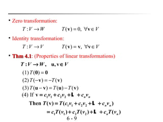
6 - 9

Zero transformation:
: , u, vT V W V→ ∈
VT ∈∀= vv ,0)(

Identity transformation:
VVT →: VT ∈∀= vvv ,)(

Thm 4.1Thm 4.1: (Properties of linear transformations)
WVT →:
00 =)((1)T
)()((2) vv TT −=−
)()()((3) vuvu TTT −=−
(4) If 1 1 2 2
1 1 2 2
1 1 2 2
v
Then (v) ( )
( ) ( ) ( )
n n
n n
n n
c v c v c v
T T c v c v c v
c T v c T v c T v
= + + +
= + + +
= + + +
L
L
L

6 - 10

Ex: (Linear transformations and bases)
Let be a linear transformation such that33
: RRT →
)4,1,2()0,0,1( −=T
)2,5,1()0,1,0( −=T
)1,3,0()1,0,0( =T
Sol:
)1,0,0(2)0,1,0(3)0,0,1(2)2,3,2( −+=−
(2,3, 2) 2 (1,0,0) 3 (0,1,0) 2 (0,0,1)
2(2, 1,4) 3(1,5, 2) 2(0,3,1)
(7,7,0)
T T T T− = + −
= − + − −
=
(T is a L.T.)
Find T(2, 3, -2).

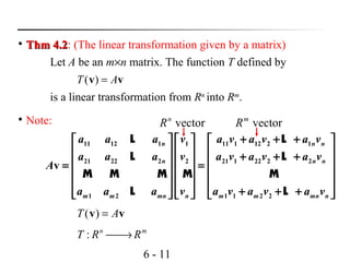
6 - 11

Thm 4.2Thm 4.2: (The linear transformation given by a matrix)
Let A be an m×n matrix. The function T defined by
vv AT =)(
is a linear transformation from Rn
into Rm
.

Note:
11 12 1 1 11 1 12 2 1
21 22 2 2 21 1 22 2 2
1 2 1 1 2 2
v
n n n
n n n
m m mn n m m mn n
a a a v a v a v a v
a a a v a v a v a v
A
a a a v a v a v a v
+ + +     
     + + +     = =
     
     
+ + +     
L L
L L
M M M M M
L L
vv AT =)(
mn
RRT →:
vectorn
R vectorm
R

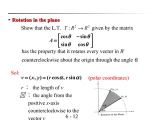
6 - 12
Show that the L.T. given by the matrix
has the property that it rotates every vector in R2
counterclockwise about the origin through the angle θ.

Rotation in the planeRotation in the plane
22
: RRT →
cos sin
sin cos
A
θ θ
θ θ
− 
=  
 
Sol:
( , ) ( cos , sin )v x y r rα α= = (polar coordinates)
r ： the length of v
 ： the angle from the
positive x-axis
counterclockwise to the

6 - 13




+
+
=




+
−
=







 −
=






 −
==
)sin(
)cos(
sincoscossin
sinsincoscos
sin
cos
cossin
sincos
cossin
sincos
)(
αθ
αθ
αθαθ
αθαθ
α
α
θθ
θθ
θθ
θθ
r
r
rr
rr
r
r
y
x
AT vv
r ： the length of T(v)
θ +α ： the angle from the positive x-axis counterclockwise
to
the vector T(v)Thus, T(v) is the vector that results from rotating the vector v
counterclockwise through the angle θ.

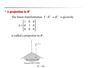
6 - 14
is called a projection in R3
.

A projection inA projection in RR33
The linear transformation is given by33
: RRT →








=
000
010
001
A

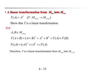
6 - 15
Show that T is a linear transformation.

A linear transformation fromA linear transformation from MMmm××nn intointo MMnn ××mm
):()( mnnm
T
MMTAAT ×× →=
Sol:
nmMBA ×∈,
)()()()( BTATBABABAT TTT
+=+=+=+
)()()( AcTcAcAcAT TT
===
Therefore, T is a linear transformation from Mm×n into Mn ×m.

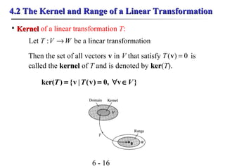
6 - 16
4.2 The Kernel and Range of a Linear Transformation4.2 The Kernel and Range of a Linear Transformation

KernelKernel of a linear transformation T:
Let be a linear transformationWVT →:
Then the set of all vectors v in V that satisfy is
called the kernelkernel of T and is denoted by kerker(T).
0)( =vT
ker( ) {v | (v) 0, v }T T V= = ∀ ∈

6 - 17

Finding the kernel of a linear transformationFinding the kernel of a linear transformation
1
3 2
2
3
1 1 2
(x) x ( : )
1 2 3
x
T A x T R R
x
 
− −   
= = →   −    
?)ker( =T
Sol:Sol:
}),,(),0,0(),,(|),,{()ker( 3
321321321 RxxxxxxxTxxxT ∈===
1 2 3( , , ) (0,0)T x x x = ⇒




=












−
−−
0
0
321
211
3
2
1
x
x
x
1
2
3
1
1
1
x t
x t t
x t
     
     ⇒ = − = −     
         
real numberker( ) { (1, 1,1) | }
span{(1, 1,1)} = Nullspace of A
T t t⇒ = − ∈
= −
.1 1 2 0 1 0 1 0
1 2 3 0 0 1 1 0
G E− − −   
→   −   

6 - 18

Thm 4.3:Thm 4.3: The kernel is a subspace of V.
The kernel of a linear transformation is a subspace of the
domain V.
WVT →:
(0) 0 (Theorem 4.1)T =QPf:Pf:
is a nonempty subset ofker( )T V∴
then.ofkernelin thevectorsbeandLet Tvu
000)()()( =+=+=+ vuvu TTT
00)()( === ccTcT uu )ker(Tc ∈⇒ u
)ker(T∈+⇒ vu
.ofsubspaceais)ker(Thus, VT

Corollary to Thm 4.3:Corollary to Thm 4.3:
0ofspacesolutionthetoequalisTofkernelThen the
)(bygivenL.Tthebe:Let
=
=→
x
xx
A
ATRRT mn
{ }
a linear transformation(x) x ( : )
( ) ( ) x | x 0, x (a subspace of )
n m
n n
T A T R R
ker T NS A A R R
= →
⇒ = = = ∀ ∈

6 - 19
Finding a basis for the kernelFinding a basis for the kernel
Let be defined by , where and5 4 5
: (x) x x is in R
1 2 0 1 1
2 1 3 1 0
1 0 2 0 1
0 0 0 2 8
T R R T A
A
→ =
− 
 
 =
 − −
 
 
Find a basis for ker(T) as a
subspace of RR55
.
Sol:
[ ] .
1 2 0 1 1 0 1 0 2 0 1 0
2 1 3 1 0 0 0 1 1 0 2 0
0
1 0 2 0 1 0 0 0 0 1 4 0
0 0 0 2 8 0 0 0 0 0 0 0
G E
A
− −   
   − −   = →
   − −
   
   
s t
1
2
3
4
5
2 2 1
2 1 2
1 0
4 0 4
0 1
x s t
x s t
xx s ts
x t
x t
− + −       
       +       
       ⇒ = = = +
       
− −       
             
is a basis
of the kernel of
{( 2, 1, 1, 0, 0)
(1, 2, 0, 4, 1)}
B and
T
= −
−

6 - 20
.:Tnnsformatiolinear traaofrangeThe WWV foecapsbusasi→

Thm 4.4Thm 4.4: The range of T is a subspace of W
Pf:Pf: (0) 0 (Thm 4.1)T =Q ( ) is a nonempty subset ofrange T W⇒
TTT ofrangein thevectorbe)(and)(Let vu
)()()()( TrangeTTT ∈+=+ vuvu
)()()( TrangecTcT ∈= uu
),( VVV ∈+⇒∈∈ vuvu
)( VcV ∈⇒∈ uu
Therefore, ( ) is a subspace ofrange T W

6 - 21
Let be the L.T. represented by
then the range of is equal to the column space of
( ) ( ) {
( ,
}
: x) xn
n
m
range T CS A
T R R
Ax
T A
T A
x R
=
= = ∀ ∈
→
⇒

Rank of a linear transformation T: V→W:
( ) the dimension of the range ofrank T T=

Nullity of a linear transformation T: V→W:
( ) the dimension of the kernel ofnullity T T=

Note:Note:
Let be the L.T. represented by ,then: (x) x
( ) ( ) dim[ ( )]
( ) ( ) dim[ ( )]
n m
T R R T A
rank T rank A CS A
nullity T nullity A NS A
→ =
= =
= =

6 - 22
Finding a basis for the range of a linear transformationFinding a basis for the range of a linear transformation
5 4 5
Let : be defined by ( ) ,where and
1 2 0 1 1
2 1 3 1 0
1 0 2 0 1
0 0 0 2 8
T R R T A R
A
→ = ∈
− 
 
 =
 − −
 
 
x x x
Find a basis for the range(T).
Sol:Sol:
.
1 2 0 1 1 1 0 2 0 1
2 1 3 1 0 0 1 1 0 2
1 0 2 0 1 0 0 0 1 4
0 0 0 2 8 0 0 0 0 0
G E
A B
− −   
   −   = → =
   − −
   
   
54321 ccccc
54321 wwwww
{ }
{ } )(,,
)(,,
421
421
ACSccc
BCSwww
forbasisais
forbasisais⇒
{ } Tofrangefor thebasisais)2,0,1,1(),0,0,1,2(),0,1,2,1( −⇒

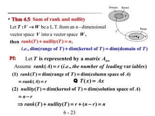
6 - 23
Let be a L.T.from an n - dimensional
vector space into a vector space
:
,
then
T V W
V W
→

Thm 4.5Thm 4.5: Sum of rank and nullity
Pf:Pf: Let is represented by a mnT matrix A
. ., dim(range of ) dim(kerne
( ) ( )
l of ) dim(domain of )
,rank T nullity T n
i e T T T+
=
=
+
Assume ( ) ( . ., var )rank A r i e the number of leading iables=
(1) ( ) dim(range of ) dim(column space of )
( )
rank T T A
rank A r
= =
= =
(2) ( ) dim(kernel of ) dim(solution space of )nullity T T A
n r
= =
= −
( ) ( ) ( )rank T nullity T r n r n⇒ + = + − =
( )T x Ax=Q

6 - 24

Finding the rank and nullity of a linear transformation
Find the rank and nullity of the L.T. define by3 3
:
1 0 2
0 1 1
0 0 0
T R R
A
→
− 
 =  
  
Sol:
( ) ( ) 2
( ) dim(domain of ) ( ) 3 2 1
rank T rank A
nullity T T rank T
= =
= − = − =

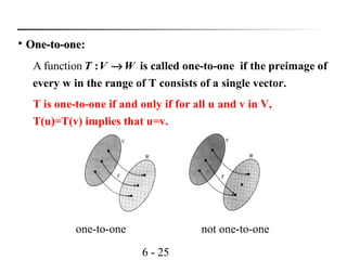
6 - 25
A function : is called one-to-one if the preimage of
every w in the range of T consists of a single vector.
T V W→

One-to-one:One-to-one:
T is one-to-one if and only if for all u and v in V,
T(u)=T(v) implies that u=v.
one-to-one not one-to-one

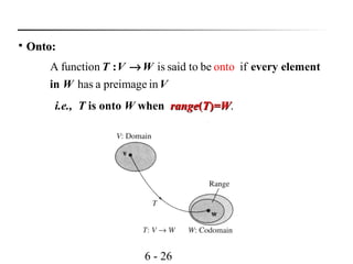
6 - 26
A function is said to be if
has a preimage in
onto: every element
in
T V W
W V
→

Onto:Onto:
i.e., T is onto W when rangerange((TT))=W=W.

6 - 27

Thm 4.6:Thm 4.6: (One-to-one linear transformation)
T is one - to -one if and
Let
only
be a L.T.,
if ( ) {0}
:
ker T
T V W
=
→
Pf: 1-1isSupposeT
0:solutiononeonlyhavecan0)(Then == vvT
.,.e ) {0i ( }ker T =
Suppose and( ) {0} ( ) ( )ker T T u T v= =
0)()()( =−=− vTuTvuT
L.T.aisT
( ) 0u v ker T u v− ∈ ⇒ − =Q is one- to -one L.T.T⇒
i.e., The addtive unit element in V is mapped onto
the additive unit element in W.

6 - 28

One-to-one and not one-to-one linear transformationOne-to-one and not one-to-one linear transformation
The L.T.( ) : given by ( )
is one-to-one.
T
m n n ma T M M T A A× ×→ =
mn
zero matrix
i.e., ker(T) = {0 }.
Because its kernel consists of only the m n×
one.-to-onenotis:ationtransformzeroThe)( 33
RRTb →
.ofalliskernelitsBecause 3
R

6 - 29

Onto linear transformationOnto linear transformation
Let be a L.T., where is finite dimensional,
then is equal to the dimension of
:
is onto iff the rank of .
T V W W
T T W
→

Thm 4.7Thm 4.7: (One-to-one and onto linear transformation)
Let be a L.T. with vector space both of
dimension then is one - to -one iff it is onto.
: and
,
T V W V W
n T
→
Pf:Pf: If is one- to -one, then and( ) {0} dim( ( )) 0T ker T ker T= =
( ) dim( ( )) dim( ( )) dim( )rank T range T n ker T n W= = − = =
onto.isly,Consequent T
dim( ( )) dim(range of ) 0ker T n T n n= − = − =
Therefore, ker(T) = {0}. is one - to -one.(from Thm 4.6)T
nWTT == )dim()ofrangedim(thenonto,isIf
( ) dim[range( )] dim[ ( )]rank T T CS A= =Note:

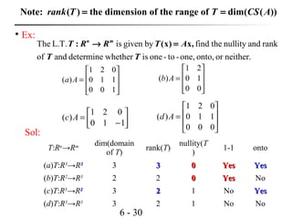
6 - 30

Ex:
The L.T. is given by find the nullity and rank
of and determine whether is one- to -one, onto, or neither.
: (x) x,n m
T R R T A
T T
→ =








=
100
110
021
)( Aa








=
00
10
21
)( Ab




−
=
110
021
)( Ac








=
000
110
021
)( Ad
Sol:
T:Rn
→Rm dim(domain
of T)
rank(T)
nullity(T
)
1-1 onto
(a)T:R3
→R33
3 33 00 YesYes YesYes
(b)T:R2
→R3
2 2 00 YesYes No
(c)T:R3
→R22
3 22 1 No YesYes
(d)T:R3
→R3
3 2 1 No No
( ) the dimension of the range of dim( ( ))rank T T CS A= =Note:

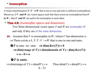
6 - 31

IsomorphismIsomorphism
A linear transformation that is one to one and onto is called an isomorphism.
Moreover, if are vector spaces such that there exists an isomorphism from
then are said to b
:
and
to , and
T V W
V W V
W V W
→
e isomorphic to each other.
Pf:Pf: .dimensionhaswhere,toisomorphicisthatAssume nVWV
onto.andonetooneisthat:L.T.aexistsThere WVT →⇒
is one - to -oneTQ
dim(range of ) dim(domain of ) dim( ( ))
0
T T Ker T
n n
⇒ = −
= − =
is onto.TQ
nWT ==⇒ )dim()ofrangedim( nWV == )dim()dim(Thus

Thm 4.8:Thm 4.8: (Isomorphic spaces and dimension)
Two finite-dimensional vector space V and W are isomorphic if
and only if they are of the same dimension.
dim( ( )) 0Ker T⇒ =

6 - 32

Ex: (Isomorphic vector spaces)
space-4)( 4
=Ra
matrices14allofspace)( 14 ×=×Mb
matrices22allofspace)( 22 ×=×Mc
lessor3degreeofspolynomialallofspace)()( 3 =xPd
)ofsubspace}(numberrealais),0,,,,{()( 5
4321 RxxxxxVe i=
The following vector spaces are isomorphic to each other.

6 - 33
4.3 Matrices for Linear Transformations4.3 Matrices for Linear Transformations
)43,23,2(),,()1( 32321321321 xxxxxxxxxxxT +−+−−+=

Three reasons for matrix representationmatrix representation of a linear transformation:
















−−
−
==
3
2
1
430
231
112
)()2(
x
x
x
AT xx

It is simpler to write.

It is simpler to read.

It is more easily adapted for computer use.

Two representationsTwo representations of the linear transformation T:R3
→R3
:

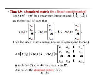
6 - 34

Thm 4.9Thm 4.9: (Standard matrixStandard matrix for a linear transformation)
1 2 n
n
Let be a linear transformation and{e ,e ,...,e }
are the basis of R such that
: n m
T R R→
r r r
1 1 1
2
2
2
2
1
1
21
1 2
2
( ) , ( ) , , ( ) ,
m
n
n
m
n
nm
a a a
a a a
T e T e T e
a a a
     
     
     = = =
     
     
     
L
M M M
Then the matrix whose columns correspond to ( )im n i T e×
is such that for every in .
A is called th standard me atrix for
(v) v v
.
n
T A R
T
=
11 12 1
21 22 2
1 2
1 2
( ) ( ) ( )
n
n
n
m m mn
a a a
a a a
A T e T e T e
a a a
 
 
 = =    
 
 
L
L
L
M M O M
L

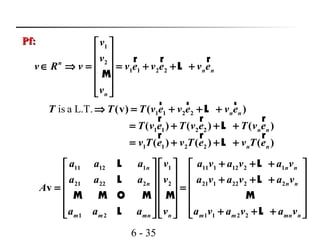
6 - 35
Pf:Pf: 1
2
1 1 2 2
n
n n
n
v
v
v R v v e v e v e
v
 
 
 ∈ ⇒ = = + + +
 
 
 
r r r
L
M
is a L.T. 1 1 2 2
1 1 2 2
1 1 2 2
(v) ( )
( ) ( ) ( )
( ) ( ) ( )
n n
n n
n n
T T T v e v e v e
T v e T v e T v e
v T e v T e v T e
⇒ = + + +
= + + +
= + + +
r r r
L
r r r
L
r r r
L
11 12 1 1 11 1 12 2 1
21 22 2 2 21 1 22 2 2
1 2 1 1 2 2
v
n n n
n n n
m m mn n m m mn n
a a a v a v a v a v
a a a v a v a v a v
A
a a a v a v a v a v
+ + +     
     + + +     = =
     
     
+ + +     
L L
L L
M M O M M M
L L

6 - 36
11 12 1
21 22 2
1 2
1 2
1 1 2 2( ) ( ) ( )
n
n
n
m m mn
n n
a a a
a a a
v v v
a a a
v T e v T e v T e
     
     
     = + + +
     
     
     
= + + +
L
M M M
L
n
RAT ineachfor)(Therefore, vvv =

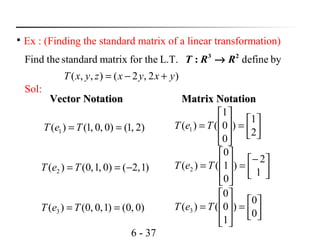
6 - 37

Ex : (Finding the standard matrix of a linear transformation)
Find the standard matrix for the L.T. define by3 2
:T R R→
)2,2(),,( yxyxzyxT +−=
Sol:
)2,1()0,0,1()( 1 == TeT
)1,2()0,1,0()( 2 −== TeT
)0,0()1,0,0()( 3 == TeT
2
1
)
0
0
1
()( 1 



=








= TeT
1
2
)
0
1
0
()( 2 


−
=








= TeT
0
0
)
1
0
0
()( 3 



=








= TeT
Vector Notation Matrix NotationVector Notation Matrix Notation

6 - 38
[ ]



 −
=
=
012
021
)()()( 321 eTeTeTA

Note:
zyx
zyx
A
012
021
012
021
++
+−
←
←



 −
=




+
−
=











 −
=








yx
yx
z
y
x
z
y
x
A
2
2
012
021
i.e., ( , , ) ( 2 ,2 )T x y z x y x y= − +

Check:

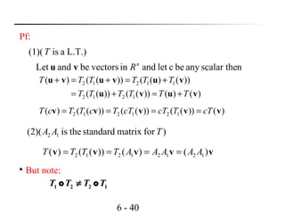
6 - 39

Composition of T1: Rn
→Rm
with T2: Rm
→Rp
:
n
RTTT ∈= vvv )),(()( 12
2 1 1, domain of domain ofT T T T T= =o

Thm 4.10:Thm 4.10: (Composition of linear transformations)
then,andmatricesstandardwith
L.T.be:and:Let
21
21
AA
RRTRRT pmmn
→→
is a .The composition L.T2 1(1) : , defined by (v) ( (v)),n p
TT R R T T→ =
is given by the matrix product 2 1(2) The standard ma fortrix A A AT A=

6 - 40
Pf:
nscalar theanybecletandinvectorsbeandLet
L.T.)ais((1)
n
R
T
vu
)formatrixstandardtheis)(2( 12 TAA
)()())(())((
))()(())(()(
1212
11212
vuvu
vuvuvu
TTTTTT
TTTTTT
+=+=
+=+=+
)())(())(())(()( 121212 vvvvv cTTcTcTTcTTcT ====
vvvvv )()())(()( 12121212 AAAAATTTT ====

But note:
1 2 2 1T T T T≠o o

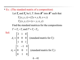
6 - 41

Ex : (The standard matrix of a composition)
Let and be L.T.from into such that3 3
1 2T T R R
),0,2(),,(1 zxyxzyxT ++=
),z,(),,(2 yyxzyxT −=
,'and
nscompositiofor thematricesstandardtheFind
2112 TTTTTT  ==
Sol:
)formatrixstandard(
101
000
012
11 TA










=
)formatrixstandard(
010
100
011
22 TA









 −
=

6 - 42
2 1The standard matrix for T T T= o
1 2The standard matrix for 'T T T= o








=















 −
==
000
101
012
101
000
012
010
100
011
12 AAA









 −
=









 −










==
001
000
122
010
100
011
101
000
012
' 21AAA

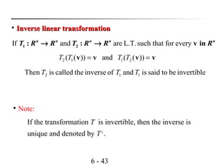
6 - 43

Inverse linear transformationInverse linear transformation
If and are L.T.such that for every1 2: : v inn n n n n
T R R T R R R→ →
))((and))(( 2112 vvvv == TTTT
invertiblebetosaidisandofinversethecalledisThen 112 TTT

Note:
If the transformation T is invertible, then the inverse is
unique and denoted by T–1
.

6 - 44

Existence of an inverse transformation
.equivalentareconditionfollowingThen the
,matrixstandardwithL.T.abe:Let ARRT nn
→

Note:
If T is invertible with standard matrix A, then the standard
matrix for T–1
is A–1
.
(1) T is invertible.
(2) T is an isomorphism.
(3) A is invertible.

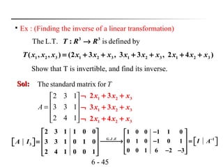
6 - 45

Ex : (Finding the inverse of a linear transformation)
The L.T. is defined by3 3
:T R R→
1 2 3 1 2 3 1 2 3 1 2 3( , , ) (2 3 , 3 3 , 2 4 )T x x x x x x x x x x x x= + + + + + +
Sol:Sol:
142
133
132
formatrixstandardThe










=A
T
1 2 3
1 2 3
1 2 3
2 3
3 3
2 4
x x x
x x x
x x x
¬ + +
¬ + +
¬ + +
3
2 3 1 1 0 0
3 3 1 0 1 0
2 4 1 0 0 1
A I
 
 =    
  
Show that T is invertible, and find its inverse.
. . 1
1 0 0 1 1 0
0 1 0 1 0 1
0 0 1 6 2 3
G J E
I A−
− 
   → − =   
 − − 

6 - 46
11
isformatrixstandardtheandinvertibleisTherefore −−
ATT
1
1 1 0
1 0 1
6 2 3
A−
− 
 = − 
 − − 
1 1 2
1 1
2 1 3
3 1 2 3
1 1 0
(v) v 1 0 1
6 2 3 6 2 3
x x x
T A x x x
x x x x
− −
− − +    
    = = − = − +    
    − − − −     
In other words,
1
1 2 3 1 2 1 3 1 2 3( , , ) ( , , 6 2 3 )T x x x x x x x x x x−
= − + − + − −

6 - 47

the matrix ofthe matrix of TT relative to the basesrelative to the bases B andB and BB''
a L.T.
1 2
1 2
: ( )
{ , , , } (a basis for )
' { , , , } (a basis for )
n
m
T V W
B v v v V
B w w w W
→
=
=
L
L
Thus, the matrix of T relative to the bases B and B' is
1 2' ' '
( ) , ( ) , , ( )n m nB B B
A T v T v T v M ×
 = ∈           L

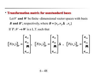
6 - 48

Transformation matrix for nonstandard basesTransformation matrix for nonstandard bases
11 12 1
21 22 2
1 2' ' '
1 2
( ) , ( ) , , ( )
n
n
nB B B
m m mn
a a a
a a a
T v T v T v
a a a
     
     
     = = =               
     
     
L
M M M
Let be finite -dimensional vector spaces with basis
respectively,where 1 2
and
and ', { , , , }n
V W
B B B v v v= L
If is a L.T.such that:T V W→

6 - 49
[ ]such that for every in'
(v) [v] v .BB
T A V=
11 12 1
21 22 2
1 2
1 2
( ) ( ) ( )
n
n
n
m m mn
a a a
a a a
A T v T v T v
a a a
 
 
 = =    
 
 
L
L
L
M M O M
L
the matrix whose i columns correspond to '
( )i B
m n T v is×   

6 - 50

Ex : (Finding a transformation matrix relative to nonstandard bases)
bydefinedL.T.abe：Let 22
RRT →
)2,(),( 212121 xxxxxxT −+=
)}1,0(),0,1{('and)}1,1(),2,1{(
basisthetorelativeofmatrixtheFind
=−= BB
T
Sol:Sol:
)1,0(3)0,1(0)3,0()1,1(
)1,0(0)0,1(3)0,3()2,1(
−=−=−
+==
T
T
[ ] [ ]' '
3 0
(1, 2) , ( 1, 1)
0 3B B
T T
   
= − =   −   
relative tothe transformation matrix and 'T B B
[ ] [ ]' '
3 0
(1, 2) ( 1, 1)
0 3B B
A T T
 
 = − =    − 

6 - 51
to findse the matrix (v),where v (2, 1)Now u A T =
)1,1(1)2,1(1)1,2( −−==v
[ ] 



−
=⇒
1
1
Bv
[ ] [ ] 



=



−



−
==⇒
3
3
1
1
30
03
)( ' BB AT vv
)3,3()1,0(3)0,1(3)( =+=⇒ vT )}1,0(),0,1{('=B
)}1,1(),2,1{( −=B
)3,3()12(2),12()1,2( =−+=T
Check:

6 - 52

Notes:Notes:
is called the matrix of relative to the basis
(1) In the special case where and ',
the matrix
V W B B
A T B
= =
relative to the basis
1 2
1 2
(2) : : the identity transformation
{ , , , }: a basis for
the matrix of
1 0 0
0 1 0
( ) , ( ) , , ( )
0 0 1
n
n nB B B
T V V
B v v v V
T B
A T v T v T v I
→
=
⇒
 
 
  = = =             
 
 
r r r
L
L
Lr r r
L
M M O M
L

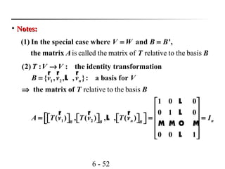
6 - 53
4.4 Transition Matrices and Similarity4.4 Transition Matrices and Similarity
a L.T.
1
2
2
1
: ( )
{ , , , }
' {
( a basis of )
(a basis of ), , , }
n
nB w
T V V
B v v
w Vw
v V
→
=
= L
L
relative to1 2( ) , ( ) , , ( ) ( matrix of )nB B B
A T v T v T v T B =            L
relative to1 2' ' '
' ( ) , ( ) , , ( ) (matrix of ')nB B B
w w wT T BA T T =            L
1 2, , , ( transition matrix from ' to )nB B B
P Bw w w B =            L
1
1 ' '2'
, , , ( transition matrix from to ')nB B B
P v v v B B−
 =            L
[ ] [ ] [ ] [ ]1
' '
v v , v vB B B B
P P−
∴ = =
[ ] [ ]
[ ] [ ]' '
(v) v
(v) ' v
B B
B B
T A
T A
=
=

6 - 54
direct
indirect

Two ways to get from to :Two ways to get from to :
' '
(1) direct
'[v] [ (v)]B BA T=
[ ] 'Bv [ ] ')( BT v
1
' '
(2) indirect
[v] [ (v)]B BP AP T−
=
1
'' '' B B B BBB P AA P−
⇒ =

6 - 55

ExEx
Sol:Sol:
[ ] '
(1, 0) (2, 1) (1, 0) (1, 1) (1,
3
1
)3 01 B
T T−
−
 
= − = ⇒ =  
 
Find the transformation matrix for 2 2
:A' T R R→
1 2 1 2 1 2( , ) (2 2 , 3 )with T x x x x x x= − − +
reletive to the basis ' {(1, 0), (1, 1)}B =
[ ] '
(1, 1) (0, 2) (1, 0) (1, 1) (1,
2
2
)2 12 B
T T
 
= = + ⇒ =  

−

−
[ ] [ ]' '
3 2
' (1, 0) (1, 1)
1 2B B
A T T
− 
 ⇒ = =    − 
[ ] [ ]' '
(I) ' (1, 0) (1, 1)B B
A T T =  

6 - 56
relative to
(II) Standard matrix for ( . ., the transformation
matrix of {(1, 0), (0, 1)})
T i e
T B =
[ ] 



−
−
==
31
22
)1,0()0,1( TTA
[ ] [ ]
1 1
The transition matrix from ' to : (1, 0) (1, 1)
0 1B B
B B P
 
 = =   
 
1 1 1
The transition matrix from to ':
0 1
B B P− − 
=  
 
relative
1
The transformation matrix of '{(1,0),(1,1)}
1 1 2 2 1 1 3 2
'
0 1 1 3 0 1 1 2
T B
A P AP− − − −       
= = =       − −       
)3,22(),( 212121 xxxxxxT +−−=with

6 - 57

Similar matrix:Similar matrix:
For square matrices A and A‘ of order n, A‘ is said to be similar to A
if there exist an invertible matrixan invertible matrix PP such that
1
'A P AP−
=

Thm 4.12:Thm 4.12: (Properties of similar matrices)
Let A, B, and C be square matrices of order n.
Then the following properties are true.
(1) A is similar to A.
(2) If A is similar to B, then B is similar to A.
(3) If A is similar to B and B is similar to C, then A is similar to C.
Pf:Pf:
nn AIIA =)1(
)(
)()2(
111
1111
−−−
−−−−
==⇒=
=⇒=
PQBAQQBPAP
PBPPPPAPBPPA

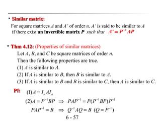
6 - 58

Ex : (A comparison of two matrices for a linear transformation)
Suppose is the matrix for relative
to the standard basis B.
3 3
1 3 0
3 1 0 :
0 0 2
A T R R
 
 = → 
 − 
)}1,0,0(),0,1,1(),0,1,1{('
basisthetorelativeformatrixtheFind
−=B
T
Sol:Sol:
[ ] [ ] [ ]
The transition matrix P from to the standard basis B is
1 1 0
(1, 1, 0) (1, 1, 0) (0, 0, 1) 1 1 0
0 0 1
B B B
B'
P
 
  = − = −   
  1 1
2 2
1 1 1
2 2
0
0
0 0 1
P−
 
 
⇒ = − 
  

6 - 59
relative to
1 1
2 2
1 1 1
2 2
''
The matrix of :
0 1 3 0 1 1 0
' 0 3 1 0 1 1 0
0 0 1 0 0 2 0 0 1
4 0 0
0 2 0
'
0 0 2
B B BB B
T
A P AP
diagonal matrix
B
−
→→
     
     = = − −     
     −    
 
 = − = 
 − 

Linear transformation.ppt

More Related Content

Linear transformation.ppt