Abstract
Purpose
To develop and evaluate a system to prescribe imaging planes for cardiac MRI based on deep learning (DL)−based localization of key anatomic landmarks.
Materials and Methods
Annotated landmarks on 892 long-axis (LAX) and 493 short-axis (SAX) cine steady-state free precession series from cardiac MR images were retrospectively collected between February 2012 and June 2017. U-Net−based heatmap regression was used for localization of cardiac landmarks, which were used to compute cardiac MRI planes. Performance was evaluated by comparing localization distances and plane angle differences between DL predictions and ground truth. The plane angulations from DL were compared with those prescribed by the technologist at the original time of acquisition. Data were split into 80% for training and 20% for testing, and results confirmed with fivefold cross-validation.
Results
On LAX images, DL localized the apex within mean 12.56 mm ± 19.11 (standard deviation) and the mitral valve (MV) within 7.68 mm ± 6.91. On SAX images, DL localized the aortic valve within 5.78 mm ± 5.68, MV within 5.90 mm ± 5.24, pulmonary valve within 6.55 mm ± 6.39, and tricuspid valve within 6.39 mm ± 5.89. On the basis of these localizations, average angle bias and mean error of DL-predicted imaging planes relative to ground truth annotations were as follows: SAX, −1.27° ± 6.81 and 4.93° ± 4.86; four chambers, 0.38° ± 6.45 and 5.16° ± 3.80; three chambers, 0.13° ± 12.70 and 9.02° ± 8.83; and two chamber, 0.25° ± 9.08 and 6.53° ± 6.28, respectively.
Conclusion
DL-based anatomic localization is a feasible strategy for planning cardiac MRI planes. This approach can produce imaging planes comparable to those defined by ground truth landmarks.
© RSNA, 2019
Summary
Deep learning−based localization is a feasible strategy for planning cardiac MRI planes.
Key Points
■ Deep learning−based approaches may improve the quality and accessibility of MRI by simplifying the imaging workflow.
■ Complex examinations that require precise placement of multiple double oblique imaging planes, like cardiac MRI, may benefit from deep learning−based anatomic localization and plane prescription.
Introduction
Cardiac MRI is the standard for quantification of cardiac volumetry, function, and blood flow (1). Cardiac MRI can be performed as a series of sequential image acquisitions, in which earlier images inform the prescription of subsequent planes. This approach is typically composed of multiple acquisitions, including a short-axis (SAX) stack and multiple long-axis (LAX) planes, requiring multiple breath holds by the patient. A key component of acquiring these images is the identification of specific cardiac structural landmarks by a physician or trained technologist. Proficient acquisition of high-quality images therefore requires extensive anatomic and technical expertise (2,3). Cardiac MRI has been predominantly limited to use in major academic institutions and subspecialty centers, which to some extent may be related to the availability of specialized expertise (4–6).
Prior attempts to help automate the prescription of cardiac imaging planes predominantly used traditional machine learning−based approaches for image analysis. Previously, Jackson et al (7) proposed a semiautomated approach with expectation maximization for planning cardiac MRI planes. However, part of this approach required the technologist to manually label blood pools. This method was developed and tested in 50 healthy patients but was not validated in a clinical population that may have had greater variation in anatomic structure. Another approach used a mesh-based segmentation model based on canonical geometry or an anatomic atlas (8,9). However, these approaches used an additional volumetric image not typically acquired at cardiac MRI.
Deep learning (DL) techniques have recently gained popularity for a variety of computer vision tasks in medical imaging ranging from disease risk stratification, segmentation of anatomic structures, and quantification of imaging features (10–13). DL has also been used for anatomic localization (14,15). For example, this method has been used previously to localize bony structures on radiographic and MR images of the hand (16). We hypothesize that this technique may be advantageously applied to localize key anatomic landmarks that define the cardiac imaging planes. Furthermore, we hypothesize that DL-based localizations of these landmarks may be sufficiently accurate to prescribe each of the cardiac imaging planes.
Materials and Methods
Patients and Data Description
With Health Insurance Portability and Accountability Act compliance and institutional review board approval, we retrospectively collected 482 cardiac MRI studies performed with a 1.5-T MRI system between February 2012 and June 2017. Within these studies there were 892 LAX cine steady-state free precession series (including 257 four-chamber, 207 three-chamber, 197 two-chamber, and 231 other LAX views) and 493 SAX cine steady-state free precession series. Of these 482 patient studies, 303 (62.86%) were in male patients and 179 (37.14%) were in female patients (age range, 12−90 years). A typical imaging protocol from our institution is in Figure E1 (supplement).
Radiology resident (T.R.) was trained by a board-certified cardiac radiologist (A.H., with 10 years of experience) to identify and annotate cardiac landmarks on each MRI series. A.H. had final approval of all ground truth annotations. LAX images were annotated for mitral valve (MV) and apex, whereas SAX stacks were annotated for aortic valve, MV, pulmonic valve, and tricuspid valve. Cine steady-state free precession images were acquired on a 1.5-T MRI system with the following parameters: mean flip angle, 54° (range, 45°−60°); 256 × 200 matrix; mean field of view, 351 mm (range, 290−440 mm); slice thickness, 8 mm (range, 5−10 mm); mean repetition time msec/echo time msec, 3.96/1 (repetition time range, 3.14−4.45 msec); and SAX stack images were acquired in intervals of 10 mm (range, 5−13 mm).
LAX Landmark Localization
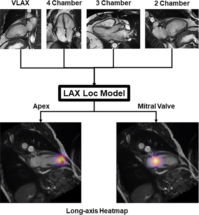
To localize the LAX landmarks (apex and MV), we implemented a two-dimensional U-Net modified for heatmap regression (16,17), trained on a variety of LAX images (Fig 1). The final convolutional layer was replaced with a linear activation and a kernel size of 1 by using L2 loss. Channel-by-channel isotropic Gaussian heatmaps centered at each localization (representing probability densities of landmark localization) were created for the apex and MV (15). DL-predicted localizations were defined by the maximal index of the predicted heatmaps.
Figure 1:
Input data used to train the long-axis (LAX) localization (Loc) model. Vertical LAX (VLAX), four-chamber, three-chamber, and two-chamber views were aggregated to train the LAX model for localization of the mitral valve and apex.
SAX Landmark Localization
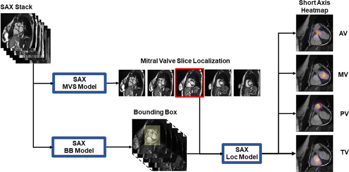
SAX stack landmark localization was decomposed into multiple two-dimensional problems (Fig 2). First, we identified the MV slice (MVS) by using an MVS localization model. Second, we created a bounding box around the heart to reduce the search space for the anatomic landmarks. Third, we created a final localization network for fine-grain anatomic localization of the aortic valve, MV, pulmonary valve, and tricuspid valve.
Figure 2:
Input data used to train short-axis (SAX) localization (Loc) models. The SAX stack images are used as inputs to train the mitral valve slice (MVS) and the bounding box (BB) models. The slice localization and BB outputs are then used to train the SAX model for localization of aortic valve (AV), mitral valve (MV), pulmonary valve (PV), and tricuspid valve (TV).
To identify the MVS, we used a previously described method with a 2.5-dimensional VGG-19/LSTM ensemble network (18–20). This redefined the MVS localization as a classification task to reduce the difficulties that arise from imbalanced data (Fig E2 [supplement]) (21,22). The MVS model was trained to classify proposal slices as either atrial or ventricular to the ground truth−labeled MVS. Spatial context was provided by adding two slices atrial and two slices ventricular to each target slice for a total of five channels. Within a given SAX stack of images, the first ventricular slice in the sorted stack was marked as the predicted MVS.
To reduce the localization search space, we implemented a 2.5-dimensional U-Net to perform a rough in-plane bounding box around the heart by using all slices of the SAX stack. Bounding box labels were defined by identifying the minimum rectangles that surround a 20-pixel in-plane border that encompassed the aortic valve, MV, pulmonary valve, and tricuspid valve landmarks.
The output of the MVS model was combined with the output of the in-plane bounding box to serve as inputs for a final localization model (Fig 2). This final localization model was implemented as a 2.5-dimensional heatmap regression model.
Plane Prescription
On the basis of the vertical LAX view, the SAX plane angle was defined as the plane orthogonal to the line between the apex and the MV landmarks (Fig E1 [supplement]). A SAX stack may therefore be prescribed at regularly spaced intervals along that line. On the basis of the SAX stack, the four-chamber plane was defined as the plane intersecting the tricuspid valve and MV, the three-chamber plane was defined as the plane intersecting the aortic valve and MV, and the two-chamber plane was defined as the plane bisecting the four-and three-chamber planes.
Model Training
DL models were each independently trained by the first author (K.B.) on a workstation running Ubuntu 16.04 and equipped with four Titan X graphics card (NVIDIA, Mountain View, Calif). We performed all DL experiments by using Keras (Keras: The Python Deep Learning Library https://keras.io/) with TensorFlow (https://www.tensorflow.org/) backend. Hyperparameters for the final models are described in Table E1 (supplement).
Model Analysis and Statistics
To assess localization accuracy, we compared ground truth expert annotation localizations with those predicted by DL, and the results were confirmed by using fivefold cross validation. For each cross-validation step, we reinitialized a blank model and independently trained it with 80% of examinations by using the remaining 20% of examinations as independent test data. Cross validation is a commonly used strategy to ensure that proposed machine learning algorithms are not dependent on the subset of training data used.
To assess plane angulation accuracy, we calculated the angle difference between DL planes and ground truth planes. As a secondary assessment of performance, we also calculated the difference between DL planes and the retrospectively identified plane prescribed by the MRI technologist at the time of image acquisition. Finally, we compared these calculated angle differences against previously reported strategies for automated plane prescription. This last comparative analysis was performed by using summary statistics reported in the previous studies. Differences in localization error and angulation error were compared by using the t test in statistical software (R; R Foundation for Statistical Computing, Vienna, Austria) with a type I error threshold (α) of .05.
Results
Landmark Localization Performance
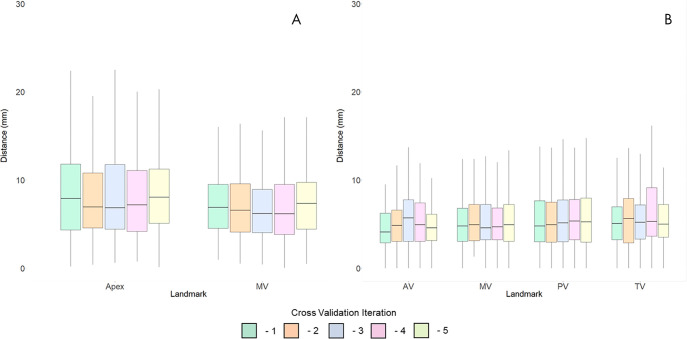
To assess localization accuracy on LAX images, we measured the distance between ground truth annotation and DL-predicted localizations. For LAX images, the mean DL localization was within 12.56 mm ± 19.11 (standard deviation) for the apex and 7.69 mm ± 6.91 for the MV (Fig 3, A). Because of the importance of vertical LAX accuracy for subsequent derivation of the SAX stack, we examined the localizations for the vertical LAX. For vertical LAX images, mean predicted localizations were within 10.20 mm ± 13.58 for the apex and 8.21 mm ± 10.71 for the MV.
Figure 3:
Distances between predicted and ground truth for the, A, long-axis and, B, short-axis localization models. Each independent iteration of cross-validation is shown in a corresponding color. AV = atrial valve, MV = mitral valve, PV = pulmonary valve, TV = tricuspid valve.
As a first step toward SAX localization, we first identified the MVS. The average distance between ground truth and predicted MVS localization was within 4.87 mm ± 8.35 on average within the 10-mm spacing between slices typically used for planar cardiac MRI at our institution. Most predicted MVS localizations (465 of 493; 94.32%) were within one slice of the labeled MVS. The second neural network was used to identify an in-plane bounding box around the heart on SAX images. These predicted segmentations had an average Dice score of 0.91 ± 0.05, relative to ground truth bounding boxes. Of these predicted bounding boxes, all (493 of 493; 100%) contained the aortic valve, 492 of 493 (99.8%) contained the MV, 490 of 493 (99.39%) contained the pulmonary valve, and 491 of 493 (99.59%) contained the tricuspid valve. After standardizing bounding boxes to native resolution, there was only one image in which the pulmonary valve and tricuspid valve localization were not contained within the input image for SAX localization. The results of the MVS localization and bounding box were then combined to create the SAX localization model. The average localization for SAX landmarks was 5.78 mm ± 5.68 for aortic valve, 5.90 mm ± 5.24 for MV, 6.55 mm ± 6.39 for pulmonary valve, and 6.39 mm ± 5.89 for tricuspid valve (Fig 3, B).
To further assess SAX landmark localizations, we compared slices that were within a single-slice error of the ground truth label (465 of 493; 94.32%), and sections that were two or more slices away (28 of 493; 5.78%). For SAX series within a single slice, average localization was as follows: aortic valve was within 5.24 mm ± 3.33 compared with 14.60 mm ± 17.66 (P < .01) for an error of two or more slices, MV was within 5.01 mm ± 3.79 compared with 12.13 mm ± 14.46 (P = .02), pulmonary valve was within 6.08 mm ± 4.99 compared with 14.03 mm ± 15.73 (P = .01), and tricuspid valve was within 5.81 mm ± 3.69 compared with 15.96 mm ± 17.19 (P < .01).
Plane Prescription Performance
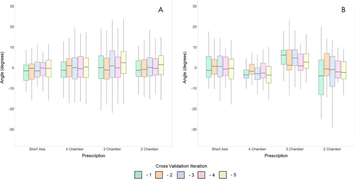
To assess the performance of landmark localizations obtained from DL, we computed plane angulations defined by these landmarks. SAX imaging planes were prescribed by using DL predictions on vertical LAX images. These plane predictions were compared against expert ground truth. For SAX plane prescription, the mean angle bias was −1.27° ± 6.81 and mean absolute angle difference was 4.93° ± 4.86 (Fig 4, A, Table 1). Similarly, LAX planes were computed from DL predictions on SAX images. For LAX plane prescription, the mean angle bias and mean absolute angle difference for the four-chamber plane were 0.38° ± 6.45 and 5.16° ± 3.80, for the three-chamber plane were 0.13° ± 12.70 and 9.02° ± 8.83, and for the two-chamber plane were 0.25° ± 9.08 and 6.53° ± 6.28. Representative images of plane prescriptions and their frequency are in Figure E3 (supplement).
Figure 4:
Comparison of plane prescriptions against, A, expert ground truth planes and, B, retrospectively matched technologist planes used during examination. Each independent cross-validation iteration is shown in a corresponding color.
Table 1:
Accuracy of Imaging Planes Prescribed by Deep Learning Compared with Expert Ground Truth and Retrospectively Matched Planes Prescribed by the MRI Technologist
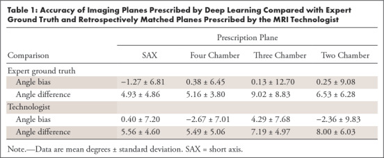
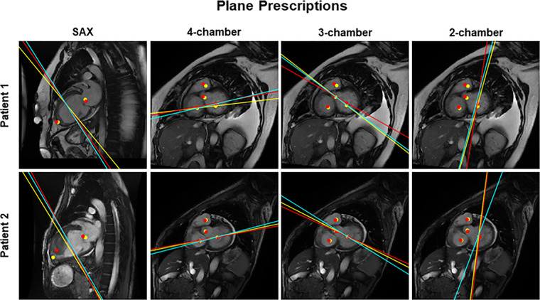
To further validate our approach of planning cardiac MRI planes by using DL-predicted landmarks, the DL planes were compared with those prescribed by a technologist at the time of acquisition (Fig 4, B, Table 1). For SAX plane prescription, the mean angle bias and mean absolute angle difference were 0.40° ± 7.20 and 5.56° ± 4.60. For LAX plane prescriptions, the mean angle bias and mean angle difference for the four-chamber plane were −2.67° ± 7.01 and 5.49° ± 5.06; for the three-chamber plane they were 4.29° ± 7.68 and 7.19° ± 4.97; and for the two-chamber plane they were −2.36° ± 9.83 and 8.00° ± 6.03. There was greater agreement and consistency between the DL prediction and technologist for the four-chamber than for the two-chamber plane. The performance of three-chamber plane prescription was in between the other LAX views. Example plane prescriptions are in Figure 5.
Figure 5:
Example images of short-axis (SAX), four-chamber, three-chamber, and two-chamber plane prescriptions from two patients. Solid lines denote the imaging planes and solid dots demarcate the localizations used to plan them. Ground truth (yellow) and the guidance system (red) are shown. The actual plane prescribed by the technologist is shown (teal). Note the large mass within the left ventricle in patient 2, which did not dramatically interfere with short-axis prescription.
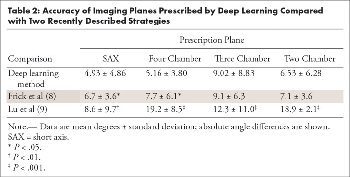
We also compared our method against recently described strategies by Frick et al (8) and Lu et al (9), and the results are in Table 2. Although our studies do not share common reference datasets, we found statistically improved SAX and four-chamber angulation relative to ground truths compared with previous methods. In addition, three-chamber and two-chamber angulations also appear improved compared with results from Lu et al.
Table 2:
Accuracy of Imaging Planes Prescribed by Deep Learning Compared with Two Recently Described Strategies
Discussion
Our study demonstrated the feasibility of using DL to localize cardiac landmarks for prescription of SAX, four-chamber, three-chamber, and two-chamber view planes. For LAX images, this was readily accomplished with a single two-dimensional U-Net modified for in-plane heatmap regression. For localization of a SAX stack, we applied a cascaded system of neural networks to localize key anatomic landmarks by first identifying the basal slice at the plane of the MV. We found that the MVS localization model correctly localized the MVS within a single slice in nearly all images (465 of 493; 94.32% of SAX inputs). More importantly, these localizations yielded imaging planes similar to those marked by a radiologist or those prescribed by a technologist at the time of image acquisition.
Previous view planning systems have been proposed for cardiac MRI. Lelieveldt et al (23) proposed planning a SAX plane by using MRI of the entire thorax. By using a deformable atlas, these authors identified the organ landmarks (including lungs, ventricles, and heart) to prescribe the SAX plane. This approach was validated by showing that clinical measurements, including ventricular mass and ejection volume, were not markedly different between acquisition approaches. However, the authors did not identify the essential four-chamber, three-chamber, and two-chamber LAX imaging planes that are necessary for the assessment of wall motion and valve function (24,25). More recently, other studies have used mesh segmentation−based approaches to plan sequences of view planes from a single three-dimensional cardiac MRI acquisition (8,9). Although promising, these approaches were developed by using a more limited test population with the use of an additional acquisition that is not typically used in many cardiac MRI workflows. Recent works have shown that DL-based approaches may benefit from the wider generalizability to other modalities and image contrasts than typically seen with traditional methods of machine learning (26). Addy et al recently presented the use of a DL-based method to plan cardiac MRI views similar to a strategy proposed by Le et al (27,28). Unlike previous efforts, we chose to assess whether we could develop a system of convolutional neural networks that could be seamlessly integrated into a typical workflow of cardiac MRI, covering the heterogeneity of heart morphologic causes and disease states seen in clinical practice.
Our study had limitations. Our study is a proof-of-concept feasibility study showing the performance of a system of neural networks for landmark localization at planar MRI. Many potential approaches exist for applying deep neural networks to solve this plane prescription problem, and it appears that DL-based landmark localization may be a feasible approach. Although the performance of this prototype system is promising, it is still relatively early in development. Room exists for further optimization and refinement of this overall strategy. In addition, there is variability in the performance of different imaging planes, with greater consistency between DL and technologists for the four-chamber view than the two-chamber view. This finding may be related to exact angle bisections done for the DL prescription, which are only visually approximated by the technologist. However, DL appears to produce planes with greater agreement with ground truth than previous methods. Future work may be required to assess the performance of such a system prospectively within a clinical workflow and determine an acceptable error range for plane prescription. To implement this strategy in practice, there are multiple additional steps that need to be implemented. For example, a SAX stack may be optimally prescribed not just from one LAX view, but perhaps two. Achieving the first LAX prescription may require additional localization on an axial or sagittal stack. Prescription of these additional acquisitions may require further development before a fully comprehensive workflow could be tested.
An important factor for overall generalizability of machine learning algorithms is the scope of the problem to be solved and the data that are ultimately used to train and test algorithm performance. We demonstrated that in a contiguous retrospective cohort of MR images from a single vendor and field strength this strategy is generally effective with few exceptions and outliers in performance. It is not yet clear whether the system will achieve similar performance on images from other MRI vendors or at 3.0 T, in which blood pool to myocardial contrast enhancement may not be relatively weaker or off-resonance banding artifacts may be present. Moreover, further work may be needed to evaluate performance of the algorithm on nongated or single-shot images, rather than the cine steady-state free precession images that were included in this study. Incorporation of these data into further training may be necessary to further generalize this method.
Nevertheless, in this study, we demonstrated that a DL-based localization approach is adequate for cardiac MRI plane prescription. It is possible that the SAX and LAX localizations may be used to sequentially optimize imaging planes, as can be performed by skilled technologists or physicians. Future work may help determine whether such a system may fully automate prescription of cardiac imaging planes. Because specialty technologist and physician training is currently a limiting factor for the availability of cardiac MRI, we believe that further development of this approach may alleviate this current barrier to access of this essential imaging modality.
SUPPLEMENTAL TABLES
SUPPLEMENTAL FIGURES
Acknowledgments
Acknowledgments
We acknowledge the support of NVIDIA Corporation for their generous donation of a Titan Xp GPU for training the deep learning networks in this research. We thank the San Diego Supercomputer Center for their donation of GPU-accelerated compute time that supported training deep learning network in this research; and the National Institute of Biomedical Imaging and Bioengineering, National Institute of General Medical Sciences, U.S. National Library of Medicine, and GE Healthcare for their generous grant support for this work.
K.B. supported by U.S. National Library of Medicine (T15 LM011271). T.R. supported by National Institute of Biomedical Imaging and Bioengineering (T32 EB005970). E.M. supported by National Institute of General Medical Sciences (T32 GM007198). A.H. supported by GE Healthcare. Study supported by NVIDIA(NVIDIA GPU Grant).
Disclosures of Conflicts of Interest: K.B. disclosed no relevant relationships. T.R. Activities related to the present article: disclosed money to author’s institution for grants from GE Medical and RSNA. Activities not related to the present article: disclosed no relevant relationships. Other relationships: disclosed patent filed with UC San Diego related to part of the work in this study. E.M. disclosed no relevant relationships. N.B. disclosed no relevant relationships. A.H. Activities related to the present article: disclosed grant from GE Healthcare. Activities not related to the present article: disclosed money paid to author for consultancy from Arterys; disclosed grants/grants pending from Bayer; disclosed payment for lectures from Bayer; disclosed patents from Stanford University and Arterys; disclosed stock/stock options from Arterys; disclosed travel/accommodations/meeting expenses unrelated to activities listed from Arterys. Other relationships: disclosed no relevant relationships.
Abbreviations:
- DL
- deep learning
- LAX
- long-axis
- MV
- mitral valve
- MVS
- MV slice
- SAX
- short-axis
References
- 1.La Gerche A, Claessen G, Van de Bruaene A, et al. Cardiac MRI: a new gold standard for ventricular volume quantification during high-intensity exercise. Circ Cardiovasc Imaging 2013;6(2):329–338. [DOI] [PubMed] [Google Scholar]
- 2.Suinesiaputra A, Bluemke DA, Cowan BR, et al. Quantification of LV function and mass by cardiovascular magnetic resonance: multi-center variability and consensus contours. J Cardiovasc Magn Reson 2015;17(1):63. [DOI] [PMC free article] [PubMed] [Google Scholar]
- 3.Ferguson M, Otto R. Cardiac MRI Prescription Planes. MedEdPORTAL 2014;10:9906. Accessed May 28, 2018. [Google Scholar]
- 4.Stokes MB, Roberts-Thomson R. The role of cardiac imaging in clinical practice. Aust Prescr 2017;40(4):151–155. [DOI] [PMC free article] [PubMed] [Google Scholar]
- 5.Crean A. Cardiovascular MR and CT in congenital heart disease. Heart 2007;93(12):1637–1647. [DOI] [PMC free article] [PubMed] [Google Scholar]
- 6.Goldfarb JW. Abstract 13092: Cardiac MRI Practice: An Analysis of 2012 and 2013 Medicare Provider Utilization and Payment Data. Circulation 2015;132(Suppl 3):13092. https://www.ahajournals.org/doi/abs/10.1161/circ.132.suppl_3.13092. [Google Scholar]
- 7.Jackson CE, Robson MD, Francis JM, Noble JA. Computerised planning of the acquisition of cardiac MR images. Comput Med Imaging Graph 2004;28(7):411–418. [DOI] [PubMed] [Google Scholar]
- 8.Frick M, Paetsch I, den Harder C, et al. Fully automatic geometry planning for cardiac MR imaging and reproducibility of functional cardiac parameters. J Magn Reson Imaging 2011;34(2):457–467. [DOI] [PubMed] [Google Scholar]
- 9.Lu X, Jolly MP, Georgescu B, et al. Automatic View Planning for Cardiac MRI Acquisition. Berlin, Germany: Springer, 2011; 479–486. [DOI] [PubMed] [Google Scholar]
- 10.Choi KJ, Jang JK, Lee SS, et al. Development and validation of a deep learning system for staging liver fibrosis by using contrast agent-enhanced CT images in the liver. Radiology 2018;289(3):688–697. [DOI] [PubMed] [Google Scholar]
- 11.Chartrand G, Cheng PM, Vorontsov E, et al. Deep learning: a primer for radiologists. RadioGraphics 2017;37(7):2113–2131. [DOI] [PubMed] [Google Scholar]
- 12.Lieman-Sifry J, Le M, Lau F, Sall S, Golden D. FastVentricle: Cardiac Segmentation with ENet. Cham, Switzerland: Springer, 2017; 127–138. [Google Scholar]
- 13.Nam JG, Park S, Hwang EJ, et al. Development and validation of deep learning-based automatic detection algorithm for malignant pulmonary nodules on chest radiographs. Radiology 2019;290(1):218–228. [DOI] [PubMed] [Google Scholar]
- 14.Pfister T, Charles J, Zisserman A. Flowing ConvNets for Human Pose Estimation in Videos. Accessed May 28, 2018.
- 15.Cao Z, Simon T, Wei SE, Sheikh Y. Realtime Multi-Person 2D Pose Estimation using Part Affinity Fields. arXiv 1611.08050 [preprint] http://arxiv.org/abs/1611.08050. Posted 2016. Accessed July 5, 2018. [DOI] [PubMed]
- 16.Payer C, Štern D, Bischof H, Urschler M. Regressing Heatmaps for Multiple Landmark Localization Using CNNs. Cham, Switzerland: Springer, 2016; 230–238. [Google Scholar]
- 17.Ronneberger O, Fischer P, Brox T. U-Net: Convolutional Networks for Biomedical Image Segmentation. arXiv [preprint] https://arxiv.org/abs/1505.04597. Posted May 18, 2015. Accessed September 27, 2018.
- 18.Simonyan K, Zisserman A. Very Deep Convolutional Networks for Large-Scale Image Recognition. arXiv [preprint] https://arxiv.org/abs/1409.1556. Posted 2015. Accessed September 27, 2018.
- 19.Hochreiter S, Schmidhuber J. Long short-term memory. Neural Comput 1997;9(8):1735–1780. [DOI] [PubMed] [Google Scholar]
- 20.Bahrami N, Retson T, Blansit K, Wang K, Hsiao A. Automated selection of myocardial inversion time with a convolutional neural network: spatial temporal ensemble myocardium inversion network (STEMI-NET). Magn Reson Med 2019;81(5):3283–3291. [DOI] [PMC free article] [PubMed] [Google Scholar]
- 21.He H, Garcia EA. Learning from imbalanced data. IEEE Trans Knowl Data Eng 2009;21(9):1263–1284. [Google Scholar]
- 22.Buda M, Maki A, Mazurowski MA. A systematic study of the class imbalance problem in convolutional neural networks. arXiv [preprint] https://arxiv.org/pdf/1710.05381.pdf. Accessed May 28, 2018. [DOI] [PubMed]
- 23.Lelieveldt BPF, van der Geest RJ, Lamb HJ, Kayser HWM, Reiber JHC. Automated observer-independent acquisition of cardiac short-axis MR images: a pilot study. Radiology 2001;221(2):537–542. [DOI] [PubMed] [Google Scholar]
- 24.Lopez-Mattei JC, Shah DJ. The role of cardiac magnetic resonance in valvular heart disease. Methodist DeBakey Cardiovasc J 2013;9(3):142–148. [DOI] [PMC free article] [PubMed] [Google Scholar]
- 25.Bloomer TN, Plein S, Radjenovic A, et al. Cine MRI using steady state free precession in the radial long axis orientation is a fast accurate method for obtaining volumetric data of the left ventricle. J Magn Reson Imaging 2001;14(6):685–692. [DOI] [PubMed] [Google Scholar]
- 26.Wang K, Mamidipalli A, Hsiao A, Sirlin C. A Convolutional Neural Network-Based Automated Hepatic-Fat Quantification Method in Non-Alcoholic Fatty Liver Disease. International Society for Magnetic Resonance in Medicine Machine Learning Workshop, 2018.
- 27.Le M, Lieman-Sifry J, Lau F, Sall S, Hsiao A, Golden D. Computationally Efficient Cardiac Views Projection Using 3D Convolutional Neural Networks. In: Cardoso MJ, Arbel T, Carneiro G, et al., eds. Deep Learning in Medical Image Analysis and Multimodal Learning for Clinical Decision Support. Cham, Switzerland: Springer International Publishing, 2017; 109–116. [Google Scholar]
- 28.Addy O, Jiang W, Overall W, Santos J, Hu B. Autonomous CMR: Prescription to Ejection Fraction in Less Than 3 Minutes. Pacific Grove, Calif: International Society for Magnetic Resonance in Medicine Machine Learning Workshop, 2018. https://cds.ismrm.org/protected/Machine18/program/videos/30950/.
Associated Data
This section collects any data citations, data availability statements, or supplementary materials included in this article.


